Yolov3 和 Yolov3-tiny目标检测算法理论与实现（TensorFlow2）

2023-11-11

文章目录

前言
一、Yolov3 和 Yolov3-tiny
1.网络结构
二、配置训练参数
- 1.目标检测数据集
- 2.设置anchor box 和classes
三、配置训练过程
四、模型预测
总结
更新进度

前言

上一篇文章神奇的目标检测已经介绍了目标检测的基础啦。目标检测呢，就是在图片中定位出目标的位置，把它“框”出来就好了。本篇文章使用Yolov3 和Yolov3-tiny，以训练VOC2007和口罩检测为例。教大家如何快速的搭建自己的目标检测平台。下面是资源链接：

内容	链接
VOC2007 数据集	链接
戴口罩数据集	链接
权重文件	链接提取码：y32m
github项目地址	链接
完整项目地址（包含所有文件）	链接提取码 jmpl

一、Yolov3 和 Yolov3-tiny

2018 年，推出了Yolov3，相比于Yolov2 最主要的改进又一下几点：
1. 加深了网络，使用Darknet53，提升了模型得检测能力。
2.使用了FPN结构（空间金字塔结构）,能增强不同大小目标的检测能力。
3.使用了focal loss，解决了样本不均和分类难得问题。
对于tiny版本来说，只使用了简单的44层卷积用作普通的特征提取，只有两个输出的yolo head （Yolov3有3个yolo head）每个网格点使用两3个anchor boxes（和Yolov3一样）。所以tiny版本检测速度是很快的哦~。
优点：检测速度快，背景误检率低，泛化性强
缺点：召回率低，定位精度较差，对于靠近或遮挡的目标，小目标检测能力弱，容易出现漏检。

1.网络结构

网络结构中包含了很多基础块，我们先实现这些基本的块，然后像搭积木一样将这些块给组装起来。每个块的用途我已经写在代码注释里了。

 #定义的卷积设置初始化方法和卷积步长和填充方式
@wraps(Conv2D)
def DarknetConv2D(*args, **kwargs):
    """Wrapper to set Darknet parameters for Convolution2D."""
    #定义卷积块
    darknet_conv_kwargs = {'kernel_regularizer': l2(5e-4)}
    darknet_conv_kwargs['padding'] = 'valid' if kwargs.get('strides')==(2,2) else 'same'
    darknet_conv_kwargs.update(kwargs)
    return Conv2D(*args, **darknet_conv_kwargs)

def DarknetConv2D_BN_Leaky(*args, **kwargs):
    #定义的卷积块包含了BN Leaky 激活函数
    """Darknet Convolution2D followed by BatchNormalization and LeakyReLU."""
    no_bias_kwargs = {'use_bias': False}
    no_bias_kwargs.update(kwargs)
    return compose(
        DarknetConv2D(*args, **no_bias_kwargs),
        BatchNormalization(),
        LeakyReLU(alpha=0.1))

def resblock_body(x, num_filters, num_blocks):
    '''A series of resblocks starting with a downsampling Convolution2D'''
    #定义 yolo 主干使用的残差快
    # Darknet uses left and top padding instead of 'same' mode
    x = ZeroPadding2D(((1,0),(1,0)))(x)
    x = DarknetConv2D_BN_Leaky(num_filters, (3,3), strides=(2,2))(x)
    for i in range(num_blocks):
        y = compose(
                DarknetConv2D_BN_Leaky(num_filters//2, (1,1)),
                DarknetConv2D_BN_Leaky(num_filters, (3,3)))(x)
        x = Add()([x,y])
    return x

def darknet_body(x):
    '''Darknent body having 52 Convolution2D layers'''
    #darknet 53
    #卷积核大小3x3 32 个卷积核
    x = DarknetConv2D_BN_Leaky(32, (3,3))(x)
    x = resblock_body(x, 64, 1)
    x = resblock_body(x, 128, 2)
    x = resblock_body(x, 256, 8)
    x = resblock_body(x, 512, 8)
    x = resblock_body(x, 1024, 4)
    return x

def make_last_layers(x, num_filters, out_filters):
    '''6 Conv2D_BN_Leaky layers followed by a Conv2D_linear layer'''
    # 这里是输入yolo，制造最后一层的代码 也就是yolo head
    x = compose(
            DarknetConv2D_BN_Leaky(num_filters, (1,1)),
            DarknetConv2D_BN_Leaky(num_filters*2, (3,3)),
            DarknetConv2D_BN_Leaky(num_filters, (1,1)),
            DarknetConv2D_BN_Leaky(num_filters*2, (3,3)),
            DarknetConv2D_BN_Leaky(num_filters, (1,1)))(x)
    y = compose(
            DarknetConv2D_BN_Leaky(num_filters*2, (3,3)),
            DarknetConv2D(out_filters, (1,1)))(x)
    return x, y

yolov3-tiny

tiny 版本网络结构比较简单，我们先来看一个图：
在这里插入图片描述
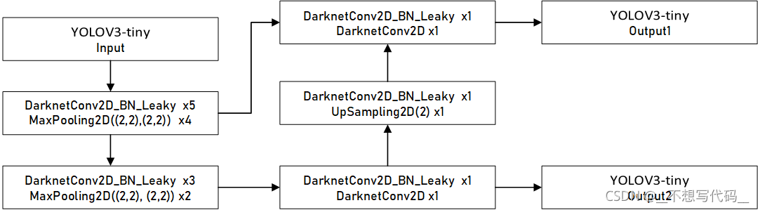
网络中就是普通的卷积核和池化，且网络很浅，网络的计算过程如箭头所示。是不是网络很简单呀~~~~~。
我们接下来看代码如何实现。

def tiny_yolo_body(inputs, num_anchors, num_classes):
	#-------------------------------------------------------------------
	# inputs 输入向量  num_anchors anchor boxes的数量 num_classes 类别数
	#------------------------------------------------------------------
    '''Create Tiny YOLO_v3 model CNN body in keras.'''
    x1 = compose(
            DarknetConv2D_BN_Leaky(16, (3,3)),
            MaxPooling2D(pool_size=(2,2), strides=(2,2), padding='same'),
            DarknetConv2D_BN_Leaky(32, (3,3)),
            MaxPooling2D(pool_size=(2,2), strides=(2,2), padding='same'),
            DarknetConv2D_BN_Leaky(64, (3,3)),
            MaxPooling2D(pool_size=(2,2), strides=(2,2), padding='same'),
            DarknetConv2D_BN_Leaky(128, (3,3)),
            MaxPooling2D(pool_size=(2,2), strides=(2,2), padding='same'),
            DarknetConv2D_BN_Leaky(256, (3,3)))(inputs)
    x2 = compose(
            MaxPooling2D(pool_size=(2,2), strides=(2,2), padding='same'),
            DarknetConv2D_BN_Leaky(512, (3,3)),
            MaxPooling2D(pool_size=(2,2), strides=(1,1), padding='same'),
            DarknetConv2D_BN_Leaky(1024, (3,3)),
            DarknetConv2D_BN_Leaky(256, (1,1)))(x1)
    y1 = compose(
            DarknetConv2D_BN_Leaky(512, (3,3)),
            DarknetConv2D(num_anchors*(num_classes+5), (1,1)))(x2)

    x2 = compose(
            DarknetConv2D_BN_Leaky(128, (1,1)),
            UpSampling2D(2))(x2)
    y2 = compose(
            Concatenate(),
            DarknetConv2D_BN_Leaky(256, (3,3)),
            DarknetConv2D(num_anchors*(num_classes+5), (1,1)))([x2,x1])

    return Model(inputs, [y1,y2])

DarknetConv2D DarknetConv2D_BN_Leaky 是使用二维卷积定义的块，可以去代码里查看，很好理解的。

yolov3

yolov3使用了残差结构和FPN, 网络较深,结构复杂，我们先来看一下他的整体网络结构：
在这里插入图片描述
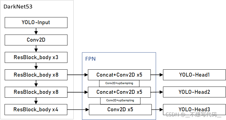
这里使用的FPN(Feature Pyramid Network) 特征金字塔如下图所示：

在目标检测中，往往会包含不用大小的目标，多层卷积后，小目标的语义丢失比较严重，使用FPN 能有效的利用多层特征信息加强浅层小目标的特征新信息，提升网络的检测能力。

def yolo_body(inputs, num_anchors, num_classes):
    """Create YOLO_V3 model CNN body in Keras."""
    #------------------------------------------------------------------
	# inputs 输入向量  num_anchors anchor boxes的数量 num_classes 类别数
	#------------------------------------------------------------------
    darknet = Model(inputs, darknet_body(inputs))
    x, y1 = make_last_layers(darknet.output, 512, num_anchors*(num_classes+5))

    x = compose(
            DarknetConv2D_BN_Leaky(256, (1,1)),
            UpSampling2D(2))(x)
    x = Concatenate()([x,darknet.layers[152].output])
    x, y2 = make_last_layers(x, 256, num_anchors*(num_classes+5))

    x = compose(
            DarknetConv2D_BN_Leaky(128, (1,1)),
            UpSampling2D(2))(x)
    x = Concatenate()([x,darknet.layers[92].output])
    x, y3 = make_last_layers(x, 128, num_anchors*(num_classes+5))
	# yolo head的输出。
    return Model(inputs, [y1,y2,y3])

代码中的 make_last_layers 是产生YOLO的输出层，对于参数：

 num_anchors*(num_classes+5)

yolo3 每个网格点有3个anchor boxes，num_achors=3 ，每个anchor box都要预测所有的类别，假设我们使用的是coco数据集有80类别，num_classes=80, 5代表框的p（框中有目标的概率），x_offset、y_offset、h和w 4个值。yolo head 中的输出维度就为 [batch_size,w,h,3x(4+1+80)]。如下图所示：
在这里插入图片描述
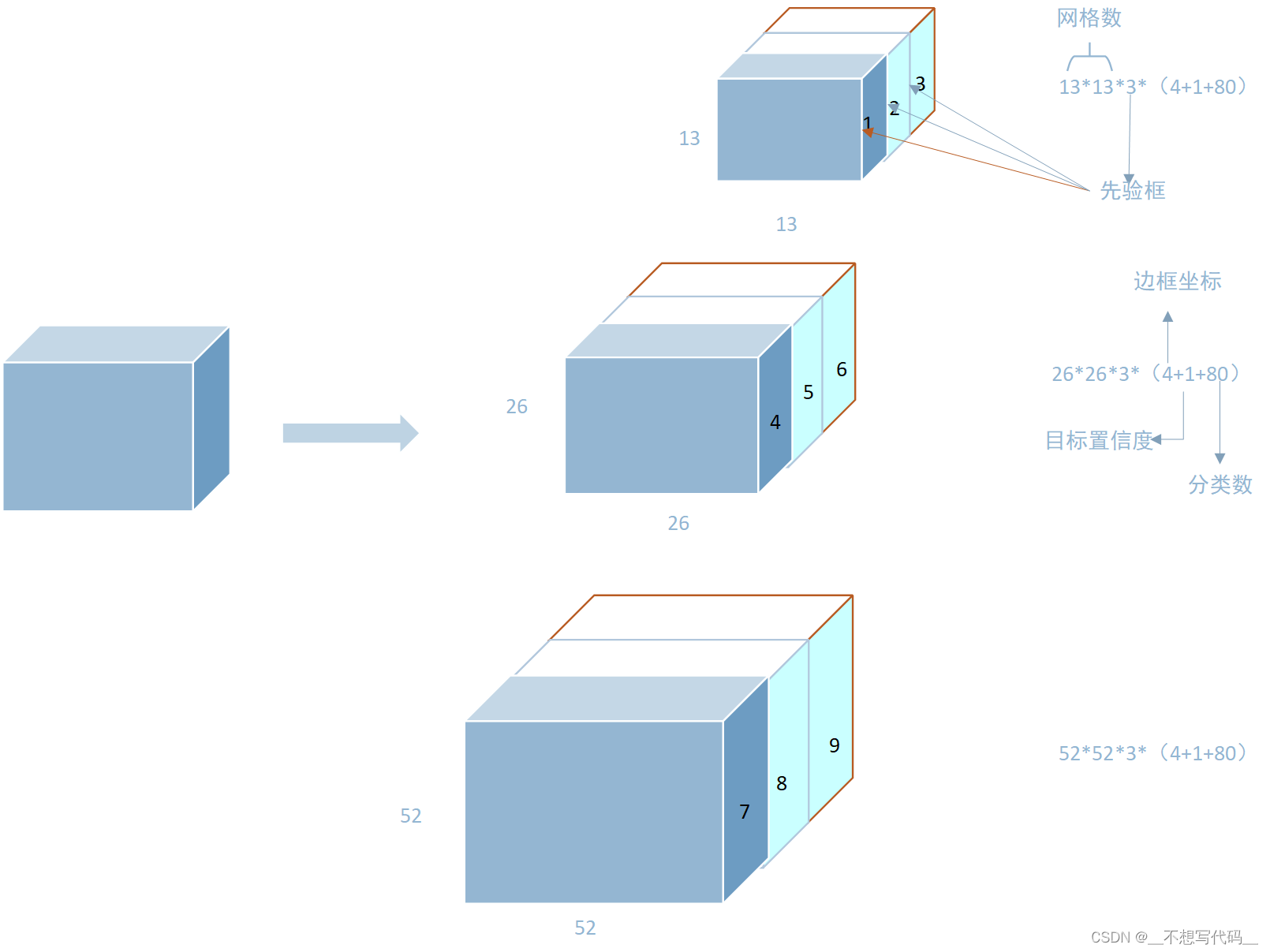
大家都会说Yolo会将图片划分为13x13，26x26, 52x52 的网格，但不是直接的物理划分，而是用这样的卷积层来表示。将每一个网格点的参数，藏在卷积特征层中，来表示物体的位置信息和类别。

网格	13*13	26*26	52*52
感受野	大（大目标）	中（中目标）	小（小目标）
先验框（coco）	116x90,156x198,373x326	30x61,62x45,59x119	10x13,16x30,33x23

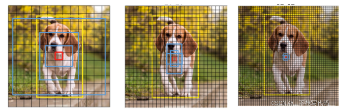
上图中黄色表示真实框, 红色表示目标中心点所在的网格。蓝色表示所设置的anchor boxes，分别检测大中小三种目标。不仅仅是以红色网格点为中心有先验框，会以每个网格点为中心都会有三个这样的先验证框。预测框数 == 网格数*锚框数。也就是总共有32x32x3+26x26x3+52x52x3个锚框。所以Yolo算法是对图片使用了"人海战术"。

框的回归

在这里插入图片描述
首先我们要明白，特征图（也就是Yolo head）表示预测框的信息：
1.坐标信息： t x , t y , t w , t h t_x,t_y,t_w,t_h tx,ty,tw,th
2.坐标置信度(有无目标)： P o b j P_obj Pobj
3.分类： p c p_c pc
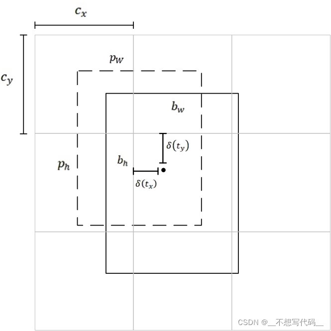
上图中锚框为长宽[Pw,Ph]，中心点为[cx,cy],预测框为[bw,bh],现在我们需要把锚框向真实框靠近需要进行两步.
第一步：中心点偏移。

其中，δ 为sigmoid 函数，bx，by为预测框中心点坐标。

第二步：宽高拉伸

这样就得到了框的长宽。我们就能还原出这样一个真实物体的框啦。

通过这样的方式就会将特征图的信息还原成，真实框啦，训练时我们训练得到的就是这些能让锚框偏移的信息。
为什么要用sigmoid 函数和exp指数呢？。因为在中心点偏移时，我们希望中心点只在它所在的网格里偏移，所以需要将其转化为0~1之间。sigmoid激活函数正好做了这件事。 宽高拉伸是因为我们宽和高的取值都是正的，那么exp函数的值域正好为0~正无穷。

二、配置训练参数

1.目标检测数据集

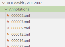
以VOC 2007 数据集为例,首先来看一下文件树：

─VOC2007
    ├─Annotations
    │	└─000005.xml
    │	└─000006.xml
    │	└─xxxx.xml	
    ├─ImageSets
    │  └─Main
    └─JPEGImages
    │	└─000005.jpg
    │	└─000006.jpg
    │	└─xxxx.jpg

每一个xml 包含同名jpg 中目标的位置以及类别，在训练时，首先要将数据通过 voc_annotation.py 转换到记事本中，方便训练时读取。记事本形式如下：

VOC2007/JPEGImages/000005.jpg（图片路径）98,267,194,383（框的位置） ,1（框中目标的类别）
VOC2007/JPEGImages/000006.jpg（图片路径）99,205,198,318（框的位置） ,1（框中目标的类别）

这样的数据是无法直接和YOLO的输出进行计算的，那么我们还需要将，这种数据编码成和yolo head 的格式一样，才能去计算loss，反向传播调整参数
通过如下函数将y_ture，转换成和y_predict 一样的形式：

def preprocess_true_boxes(true_boxes, input_shape, anchors, num_classes):
    '''Preprocess true boxes to training input format
    Parameters
    ----------
    	true_boxes: array, shape=(m, T, 5)
        Absolute x_min, y_min, x_max, y_max, class_id relative to input_shape.
    input_shape: array-like, hw, multiples of 32
    anchors: array, shape=(N, 2), wh
    num_classes: integer
    Returns
    -------
    y_true: list of array, shape like yolo_outputs, xywh are reletive value

    '''
    assert (true_boxes[..., 4]<num_classes).all(), 'class id must be less than num_classes'
    num_layers = len(anchors)//3 # default setting
    anchor_mask = [[6,7,8], [3,4,5], [0,1,2]] if num_layers==3 else [[3,4,5], [1,2,3]]

    true_boxes = np.array(true_boxes, dtype='float32')
    input_shape = np.array(input_shape, dtype='int32')
    boxes_xy = (true_boxes[..., 0:2] + true_boxes[..., 2:4]) // 2
    boxes_wh = true_boxes[..., 2:4] - true_boxes[..., 0:2]
    true_boxes[..., 0:2] = boxes_xy/input_shape[::-1]
    true_boxes[..., 2:4] = boxes_wh/input_shape[::-1]

    m = true_boxes.shape[0]
    grid_shapes = [input_shape//{0:32, 1:16, 2:8}[l] for l in range(num_layers)]
    y_true = [np.zeros((m,grid_shapes[l][0],grid_shapes[l][1],len(anchor_mask[l]),5+num_classes),
        dtype='float32') for l in range(num_layers)]

    # Expand dim to apply broadcasting.
    anchors = np.expand_dims(anchors, 0)
    anchor_maxes = anchors / 2.
    anchor_mins = -anchor_maxes
    valid_mask = boxes_wh[..., 0]>0

    for b in range(m):
        # Discard zero rows.
        wh = boxes_wh[b, valid_mask[b]]
        if len(wh)==0: continue
        # Expand dim to apply broadcasting.
        wh = np.expand_dims(wh, -2)
        box_maxes = wh / 2.
        box_mins = -box_maxes

        intersect_mins = np.maximum(box_mins, anchor_mins)
        intersect_maxes = np.minimum(box_maxes, anchor_maxes)
        intersect_wh = np.maximum(intersect_maxes - intersect_mins, 0.)
        intersect_area = intersect_wh[..., 0] * intersect_wh[..., 1]
        box_area = wh[..., 0] * wh[..., 1]
        anchor_area = anchors[..., 0] * anchors[..., 1]
        iou = intersect_area / (box_area + anchor_area - intersect_area)

        # Find best anchor for each true box
        best_anchor = np.argmax(iou, axis=-1)

        for t, n in enumerate(best_anchor):
            for l in range(num_layers):
                if n in anchor_mask[l]:
                    i = np.floor(true_boxes[b,t,0]*grid_shapes[l][1]).astype('int32')
                    j = np.floor(true_boxes[b,t,1]*grid_shapes[l][0]).astype('int32')
                    k = anchor_mask[l].index(n)
                    c = true_boxes[b,t, 4].astype('int32')
                    y_true[l][b, j, i, k, 0:4] = true_boxes[b,t, 0:4]
                    y_true[l][b, j, i, k, 4] = 1
                    y_true[l][b, j, i, k, 5+c] = 1
    #print(y_true.shape)
    return y_true

数据集放置如下图所示：
在这里插入图片描述

2.设置anchor box 和classes

Yolo 中的anchor boxes 是通过数据集中框的大小通过kmeans聚类而来，yolov3 有三个输出，每个网格预测3个，所以 Kmeans中的K设置9，如果是tiny版本的话，就设置为6。代码如下：

import numpy as np
"""
Kmeans 聚类算法， 根据 数据集中的xml 文件 聚类出是和目标的anchor boxes
"""
class YOLO_Kmeans:

    def __init__(self, cluster_number, filename):
        self.cluster_number = cluster_number
        self.filename =filename

    def iou(self, boxes, clusters):  # 1 box -> k clusters
        n = boxes.shape[0]
        k = self.cluster_number

        box_area = boxes[:, 0] * boxes[:, 1]
        box_area = box_area.repeat(k)
        box_area = np.reshape(box_area, (n, k))

        cluster_area = clusters[:, 0] * clusters[:, 1]
        cluster_area = np.tile(cluster_area, [1, n])
        cluster_area = np.reshape(cluster_area, (n, k))

        box_w_matrix = np.reshape(boxes[:, 0].repeat(k), (n, k))
        cluster_w_matrix = np.reshape(np.tile(clusters[:, 0], (1, n)), (n, k))
        min_w_matrix = np.minimum(cluster_w_matrix, box_w_matrix)

        box_h_matrix = np.reshape(boxes[:, 1].repeat(k), (n, k))
        cluster_h_matrix = np.reshape(np.tile(clusters[:, 1], (1, n)), (n, k))
        min_h_matrix = np.minimum(cluster_h_matrix, box_h_matrix)
        inter_area = np.multiply(min_w_matrix, min_h_matrix)

        result = inter_area / (box_area + cluster_area - inter_area)
        return result

    def avg_iou(self, boxes, clusters):
        accuracy = np.mean([np.max(self.iou(boxes, clusters), axis=1)])
        return accuracy

    def kmeans(self, boxes, k, dist=np.median):
        box_number = boxes.shape[0]
        distances = np.empty((box_number, k))
        last_nearest = np.zeros((box_number,))
        np.random.seed()
        clusters = boxes[np.random.choice(
            box_number, k, replace=False)]  # init k clusters
        while True:

            distances = 1 - self.iou(boxes, clusters)

            current_nearest = np.argmin(distances, axis=1)
            if (last_nearest == current_nearest).all():
                break  # clusters won't change
            for cluster in range(k):
                clusters[cluster] = dist(  # update clusters
                    boxes[current_nearest == cluster], axis=0)

            last_nearest = current_nearest

        return clusters

    def result2txt(self, data):
        f = open("yolo_anchors1.txt", 'w') # 这里是生存achor后保存的路径
        row = np.shape(data)[0]
        for i in range(row):
            if i == 0:
                x_y = "%d,%d" % (data[i][0], data[i][1])
            else:
                x_y = ", %d,%d" % (data[i][0], data[i][1])
            f.write(x_y)
        f.close()

    def txt2boxes(self):
        f = open(self.filename, 'r')
        dataSet = []
        for line in f:
            infos = line.split(" ")
            length = len(infos)
            for i in range(1, length):
                width = int(infos[i].split(",")[2]) - \
                    int(infos[i].split(",")[0])
                height = int(infos[i].split(",")[3]) - \
                    int(infos[i].split(",")[1])
                dataSet.append([width, height])
        result = np.array(dataSet)
        f.close()
        return result

    def txt2clusters(self):
        all_boxes = self.txt2boxes()
        result = self.kmeans(all_boxes, k=self.cluster_number)
        result = result[np.lexsort(result.T[0, None])]
        self.result2txt(result)
        print("K anchors:\n {}".format(result))
        print("Accuracy: {:.2f}%".format(
            self.avg_iou(all_boxes, result) * 100))

#通过聚类方法设置数据集中合适的框
if __name__ == "__main__":
    cluster_number =9 #聚类框的个数 6 或者 9
    filename = r"2007_train.txt" # 指定train.txt的路劲
    kmeans = YOLO_Kmeans(cluster_number, filename)
    kmeans.txt2clusters()

当然也可以使用yolo中默认的achor box的大小。
classes.txt 是声明你目标中所有的类别，以戴口罩数据集为例

without_mask
with_mask
mask_weared_incorrect

文本中书写的类别要和你xml 文件中所写类别保持一致，才能正确索引。

三、配置训练过程

训练过程需要配置的东西，就是之前的数据准备。输入模型即可。
训练过错内存溢出，记得吧batch_size 改小一点，yolo完整版的话一般设置为8比较好
代码：

def train():
    # 你的 数据集文件路劲
    train_annotation_path = r"2007_train.txt" # 生存的数据索引txt文本
    val_annotation_path = r"2007_val.txt"

    anchors_path = r"model_data\mask_anchor.txt" # 生成的anchor
    classes_path = r"model_data\mask_classes.txt" #自己数据集的类别
    log_dir = "logs/tiny_log/"
    weights_dir = "weights/"
    class_names = get_classes(classes_path)
    num_classes = len(class_names)
    anchors = get_anchors(anchors_path)

    input_shape = (416, 416)  #  必须是32的 倍数  yolo 的设定

	# tiny 版本
    model = create_tiny_model(
        input_shape=input_shape,
        anchors=anchors,
        num_classes=num_classes,
        freeze_body=2,
        weights_path="model_data\yolov3-tiny.h5",
    )
    ''''
     # yolo v3 的完整版本 ，
    model = create_model(
        input_shape=input_shape,
        anchors=anchors,
        num_classes=num_classes,
        # freeze_body=0,
        weights_path="model_data\yolov3.h5",
    )
    '''
    print(len(model.layers))
    logging = TensorBoard(log_dir=log_dir)
    checkpoint = ModelCheckpoint(
        weights_dir + "ep{epoch:03d}-loss{loss:.3f}-val_loss{val_loss:.3f}.h5",
        monitor="val_loss",
        save_weights_only=True,
        save_best_only=True,
        period=3,
    )
    reduce_lr = ReduceLROnPlateau(monitor="val_loss", factor=0.1, patience=3, verbose=1)
    early_stopping = EarlyStopping(
        monitor="val_loss", min_delta=0, patience=10, verbose=1
    )

    # 读取数据集对应的 .txt 文件
    with open(train_annotation_path) as f:
        train_lines = f.readlines()
    with open(val_annotation_path) as f:
        val_lines = f.readlines()
    num_train = len(train_lines)
    num_val = len(val_lines)

    # 配置训练参数
    Freeze_Train = True
    # ------------------------------------------------------------
    # 先冻结一定网络层进行训练，这样训练比较快 ,得到一个loss稳定的model
    # -------------------------------------------------------------
    if Freeze_Train:
        batch_size = 32
        model.compile(
            optimizer=Adam(1e-3),
            loss={# use custom yolo_loss Lambda layer.
            "yolo_loss": lambda y_true, y_pred: y_pred}
        )
        print("Train on {} samples, val on {} samples, with batch size {}.".format(num_train, num_val, batch_size))
        model.fit(
            data_generator_wrapper(train_lines,batch_size,input_shape,anchors,num_classes),
            steps_per_epoch=max(1,num_train//batch_size),
            validation_data=data_generator_wrapper(val_lines,batch_size,input_shape,anchors,num_classes),
            validation_steps=max(1,num_val//batch_size),
            epochs=50,
            initial_epoch=0,
            callbacks=[logging,checkpoint]
        )
        model.save_weights(weights_dir+'trained_weights_stage_1.h5')
     #-----------------------------------------------------------------
     # 解冻所有层，并调小学习率训练
     #-----------------------------------------------------------------
    if True:
        for i in range(len(model.layers)): model.layers[i].trainable = True
        model.compile(optimizer=Adam(lr=1e-4), loss={'yolo_loss': lambda y_true, y_pred: y_pred}) # recompile to apply the change
        print('Unfreeze all of the layers.')

        batch_size = 32 # note that more GPU memory is required after unfreezing the body
        print('Train on {} samples, val on {} samples, with batch size {}.'.format(num_train, num_val, batch_size))
        model.fit_generator(data_generator_wrapper(train_lines, batch_size, input_shape, anchors, num_classes),
            steps_per_epoch=max(1, num_train//batch_size),
            validation_data=data_generator_wrapper(val_lines, batch_size, input_shape, anchors, num_classes),
            validation_steps=max(1, num_val//batch_size),
            epochs=100,
            initial_epoch=50,
            callbacks=[logging, checkpoint, reduce_lr, early_stopping])
        model.save_weights(log_dir + 'trained_weights_final.h5')


if __name__=='__main__':
    train()

上述就是训练过程了，训练时，
注意：
使用model 时，tiny 和YOLOv3 achor 不一样，一个是6 类一个是9类，记得更换。
tips:训练过错先冻结一部分层去训练，这样训练比较快，当损失稳定之后，使用更小的学习率去，趋势模型收敛更好。
训练结果如下：
在这里插入图片描述
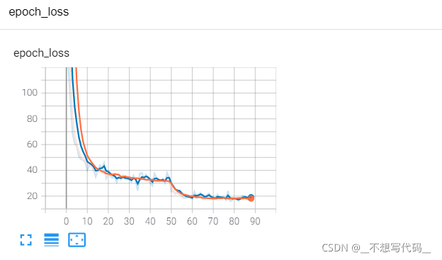
可以看出收敛效果还是相当不错的。。。。

四、模型预测

模型预测，将图片输入到保存的模型当中，如果输出一个跟yolo head 一样的维度，很显然这个时候我们是无法获图片的类别还有框的，那么需要通过解码，拿到我们有用的数据。这个工作在项目中的yolo.py 中实现。

#这里不给出全部代码了，但在预测是，网络的权重文件 achor boxes 和classes 要保持一直，在文件中这个位置配置
_defaults = {
        # ----------------------------------
        # 模型路径, anchor路径，class 路径， 
        # sorce 一本设为0.5  置信度阈值 iou 
        #  输入图片大小 一般是13 的倍数
        #   gpu 1
        #  遇上维度 不匹配问题  可能是训练时 忘记让model_path 和class_path 对应 
        # -----------------------------------
        "model_path": r"logs\yolov3_log\trained_weights_final.h5",
        "anchors_path": "model_data\mask_anchor.txt",
        "classes_path": "model_data\mask_classes.txt",
        "score": 0.3, # 置信度 ，自己改大一点
        "iou": 0.3,
        "model_image_size": (416, 416),
        "gpu_num": 1, # 这里使用1 ，多gpu 由于TensorFlow 版本问题 我给注解掉了
    }

模型预测完整代码：

import time

import cv2
import numpy as np
import tensorflow as tf
from PIL import Image
from yolo import YOLO,detect_video
import os
from tqdm import tqdm
def predict():
    #-------------------------------------------------------------
    # 新建 yolo 对象，使用模型权重路径，以及其他参数，到yolo.py 中更改
    # predict_model 为 img 预测图片， video  输入为视频，记得更改视频路劲   video_path 为 0 时调用摄像头  为视频路径时 读取视频
    # predict_model 为 dir_predict 时输入为存放图片的路径 ，预测完成后 放入out_img 使用时记得修改路劲
    # 要预测  指定类别是 ，可以设置好重新训练模型，或者进入detect_image 修改参数 if predicted_classes='car'
    #--------------------------------------------------------------
    yolo=YOLO()  
    predict_model='dir_predict'

    video_path= 0
    video_save_path=""

    dir_img_input='img/'
    dir_save_path='out_img/'
    if predict_model=='img':
        while(True):
            img=input('Input image filename:')
            try:
                image=Image.open(img)
            except:
                print('Open Image Error！ Please Try Again')
                continue
            else:
                out_image=yolo.detect_image(image)
                out_image.show()
    elif predict_model=='video':
        detect_video(yolo,video_path,video_save_path) # 可以获取fps
    
    elif predict_model=='dir_predict':
        #---------------------------------
        #拿到所有图片 通过detect image 检测
        #-------------------------------
        imgs=os.listdir(dir_img_input)
        for img_name in tqdm(imgs):
             if img_name.lower().endswith(('.bmp', '.dib', '.png', '.jpg', '.jpeg', '.pbm', '.pgm', '.ppm', '.tif', '.tiff')):
                image_path  = os.path.join(dir_img_input, img_name)
                image       = Image.open(image_path)
                r_image     = yolo.detect_image(image)
                if not os.path.exists(dir_save_path):
                    os.makedirs(dir_save_path)
                r_image.save(os.path.join(dir_save_path, img_name)) 
    else:
           raise AssertionError("Please specify the correct mode: 'img', 'video', 'dir_predict'.")
if __name__=='__main__':
    predict()

使用方法写在注释里了。支持视频，图片文件夹
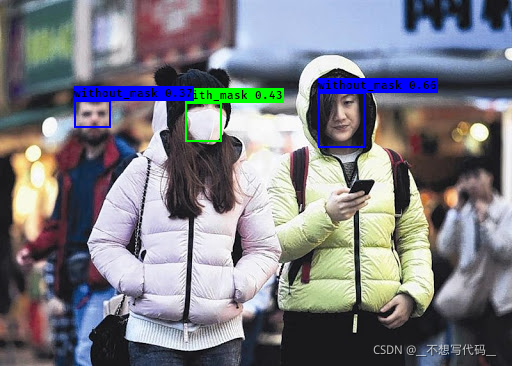
检测结果：
在这里插入图片描述

总结

目标检测网络结构，其实跟图像分类差不多，但对数据读取过程，编码解码过程比较复杂，对于这个过程，我掌握不是很多，所以就不在这里讲解了。
目标检测训练比较难，数据标注比较麻烦。后面可能会出一期视频，教大家如何配置。所有代码和资源均会上传，写代码不易，欢迎点赞~

更新进度

2022/1/15日。重置了YOLOV3 Anchor 框的设置理论讲解。接下来完成anchor boxes 框是如何回归及loss 计算过程。
2022/2/5日。添加了anchor boxes 和预测框之间的计算过程。
2022/2/14日，更改冗余错误，接下来会去重置代码。

本文内容由网友自发贡献，版权归原作者所有，本站不承担相应法律责任。如您发现有涉嫌抄袭侵权的内容，请联系:hwhale#tublm.com(使用前将#替换为@)