淘宝用户行为分析及可视化
分析背景
-
对淘宝2014年11月18至12月18日用户行为进行分析,该数据集包含了1200+万行,数据字段详解:
- user_id: 用户ID
- item_id: 商品ID
- behavior_type: 用户操作行为。1-点击,2-收藏,3-加入购物车,4-支付
- user_geohash: 用户地理位置(经过脱敏处理)
- item_category: 品类ID,商品所属种类
- time: 操作时间
-
数据来源:https://tianchi.aliyun.com/dataset/dataDetail?dataId=46
-
旨在针对电商用户行为进行分析
明确问题
- 了解淘宝的日浏览量和日独立用户数
- 淘宝用户的消费及复购行为
- 淘宝平台各种用户行为之间的转化率
- 留存率分析
- 利用二八理论分析淘宝主要商品的价值
- 建立RFM模型对用户进行分类
import pandas as pd
import numpy as np
import matplotlib.pyplot as plt
from pyecharts.charts import Bar, Funnel
from pyecharts import options as opts

# 解决suptitle报警问题
# import matplotlib
# matplotlib.use("TkAgg")

# 设置主题
plt.style.use('ggplot')

# 解决中文字符显示
plt.rcParams['font.sans-serif'] = ['SimHei']
plt.rcParams['axes.unicode_minus'] = False
读取和理解数据
data = pd.read_csv('tianchi_mobile_recommend_train_user.csv', dtype=str, encoding='utf-8')
data.info()
<class 'pandas.core.frame.DataFrame'>
RangeIndex: 12256906 entries, 0 to 12256905
Data columns (total 6 columns):
 #   Column         Dtype
---  ------         -----
 0   user_id        object
 1   item_id        object
 2   behavior_type  object
 3   user_geohash   object
 4   item_category  object
 5   time           object
dtypes: object(6)
memory usage: 561.1+ MB
data.head()
|
user_id |
item_id |
behavior_type |
user_geohash |
item_category |
time |
| 0 |
98047837 |
232431562 |
1 |
NaN |
4245 |
2014-12-06 02 |
| 1 |
97726136 |
383583590 |
1 |
NaN |
5894 |
2014-12-09 20 |
| 2 |
98607707 |
64749712 |
1 |
NaN |
2883 |
2014-12-18 11 |
| 3 |
98662432 |
320593836 |
1 |
96nn52n |
6562 |
2014-12-06 10 |
| 4 |
98145908 |
290208520 |
1 |
NaN |
13926 |
2014-12-16 21 |
数据预处理
# 统计缺失值
data.apply(lambda x: sum(x.isnull()))
user_id                0
item_id                0
behavior_type          0
user_geohash     8334824
item_category          0
time                   0
dtype: int64
# 统计缺失率
data.apply(lambda x: sum(x.isnull()) / len(x))
user_id          0.00000
item_id          0.00000
behavior_type    0.00000
user_geohash     0.68001
item_category    0.00000
time             0.00000
dtype: float64
# 分割日期,转换形式
data['date'] = data['time'].str[:-3]
data['hour'] = data['time'].str[-2:].astype(int)
data['date'] = pd.to_datetime(data['date'])
data['time'] = pd.to_datetime(data['time'])
data.head()
|
user_id |
item_id |
behavior_type |
user_geohash |
item_category |
time |
date |
hour |
| 0 |
98047837 |
232431562 |
1 |
NaN |
4245 |
2014-12-06 02:00:00 |
2014-12-06 |
2 |
| 1 |
97726136 |
383583590 |
1 |
NaN |
5894 |
2014-12-09 20:00:00 |
2014-12-09 |
20 |
| 2 |
98607707 |
64749712 |
1 |
NaN |
2883 |
2014-12-18 11:00:00 |
2014-12-18 |
11 |
| 3 |
98662432 |
320593836 |
1 |
96nn52n |
6562 |
2014-12-06 10:00:00 |
2014-12-06 |
10 |
| 4 |
98145908 |
290208520 |
1 |
NaN |
13926 |
2014-12-16 21:00:00 |
2014-12-16 |
21 |
data.dtypes
user_id                  object
item_id                  object
behavior_type            object
user_geohash             object
item_category            object
time             datetime64[ns]
date             datetime64[ns]
hour                      int32
dtype: object
data.sort_values(by='time', ascending=True, inplace=True)
data.reset_index(drop=True, inplace=True)
data.head()
|
user_id |
item_id |
behavior_type |
user_geohash |
item_category |
time |
date |
hour |
| 0 |
73462715 |
378485233 |
1 |
NaN |
9130 |
2014-11-18 |
2014-11-18 |
0 |
| 1 |
36090137 |
236748115 |
1 |
NaN |
10523 |
2014-11-18 |
2014-11-18 |
0 |
| 2 |
40459733 |
155218177 |
1 |
NaN |
8561 |
2014-11-18 |
2014-11-18 |
0 |
| 3 |
814199 |
149808524 |
1 |
NaN |
9053 |
2014-11-18 |
2014-11-18 |
0 |
| 4 |
113309982 |
5730861 |
1 |
NaN |
3783 |
2014-11-18 |
2014-11-18 |
0 |
# 对字符型数据进行统计,describe()理解include参数
data.describe(include=['object'])
|
user_id |
item_id |
behavior_type |
user_geohash |
item_category |
| count |
12256906 |
12256906 |
12256906 |
3922082 |
12256906 |
| unique |
10000 |
2876947 |
4 |
575458 |
8916 |
| top |
36233277 |
112921337 |
1 |
94ek6ke |
1863 |
| freq |
31030 |
1445 |
11550581 |
1052 |
393247 |
数据分析与可视化
用户行为分析
日PV和日UV
pv_daily = data.groupby('date').count()[['user_id']].rename(columns={'user_id':'pv'})
pv_daily.head()
|
pv |
| date |
|
| 2014-11-18 |
366701 |
| 2014-11-19 |
358823 |
| 2014-11-20 |
353429 |
| 2014-11-21 |
333104 |
| 2014-11-22 |
361355 |
# 每日独立访客量
uv_daily = data.groupby('date')[['user_id']].apply(lambda x: x.drop_duplicates().count()).rename(columns={'user_id':'uv'})
uv_daily.head()
|
uv |
| date |
|
| 2014-11-18 |
6343 |
| 2014-11-19 |
6420 |
| 2014-11-20 |
6333 |
| 2014-11-21 |
6276 |
| 2014-11-22 |
6187 |
# 合并
pv_uv_daily = pd.concat([pv_daily, uv_daily], axis=1)
pv_uv_daily.head()
|
pv |
uv |
| date |
|
|
| 2014-11-18 |
366701 |
6343 |
| 2014-11-19 |
358823 |
6420 |
| 2014-11-20 |
353429 |
6333 |
| 2014-11-21 |
333104 |
6276 |
| 2014-11-22 |
361355 |
6187 |
PV与UV相关性
# pv与uv的相关性,method可以是相关性{spearman、pearson(默认)} 非相关性{kendall}
pv_uv_daily.corr(method='pearson')
|
pv |
uv |
| pv |
1.000000 |
0.920602 |
| uv |
0.920602 |
1.000000 |
可视化
plt.figure(figsize=(9, 9), dpi=70)
plt.subplot(211)
plt.plot(pv_daily, color='red')
plt.title('每日访问量', pad=10)
plt.xticks(rotation=45)
plt.grid(b=False)
plt.subplot(212)
plt.plot(uv_daily, color='green')
plt.title('每日访问用户数', pad=10)
plt.xticks(rotation=45)
plt.suptitle('PV和UV变化趋势', fontsize=20)
plt.subplots_adjust(hspace=0.5)
plt.grid(b=False)
plt.show()
时PV和时UV
pv_hour = data.groupby('hour').count()[['user_id']].rename(columns={'user_id':'pv'})
uv_hour = data.groupby('hour')[['user_id']].apply(lambda x: x.drop_duplicates().count()).rename(columns={'user_id':'uv'})
pv_uv_hour = pd.concat([pv_hour, uv_hour], axis=1)
pv_uv_hour.head()
|
pv |
uv |
| hour |
|
|
| 0 |
517404 |
5786 |
| 1 |
267682 |
3780 |
| 2 |
147090 |
2532 |
| 3 |
98516 |
1937 |
| 4 |
80487 |
1765 |
相关性
# 相关性
pv_uv_hour.corr(method='spearman')
|
pv |
uv |
| pv |
1.000000 |
0.903478 |
| uv |
0.903478 |
1.000000 |
可视化
fig = plt.figure(figsize=(9, 7), dpi=70)
fig.suptitle('PV和UV变化趋势', y=0.93, fontsize=18)
ax1 = fig.add_subplot(111)
ax1.plot(pv_hour, color='blue', label='每小时访问量')
ax1.set_xticks(list(np.arange(0,24)))
ax1.legend(loc='upper center', fontsize=12)
ax1.set_ylabel('访问量')
ax1.set_xlabel('小时')
ax1.grid(False)
ax2 = ax1.twinx()
ax2.plot(uv_hour, color='red', label='每小时访问用户数')
ax2.legend(loc='upper left', fontsize=12)
ax2.set_ylabel('访问用户数')
ax2.grid(False)
fig.show()
D:\ProgramData\Anaconda3\lib\site-packages\ipykernel_launcher.py:15: UserWarning: Matplotlib is currently using module://ipykernel.pylab.backend_inline, which is a non-GUI backend, so cannot show the figure.
  from ipykernel import kernelapp as app
不同行为类型用户PV分析
# data.groupby(['date', 'behavior_type'])[['user_id']].count().reset_index().rename(columns={'user_id':'pv'})
diff_behavior_pv = data.pivot_table(columns='behavior_type', index='date', values='user_id', aggfunc='count').rename(columns={'1':'click', '2':'collect', '3':'addToCart', '4':'pay'}).reset_index()
diff_behavior_pv.describe()
| behavior_type |
click |
collect |
addToCart |
pay |
| count |
31.000000 |
31.000000 |
31.000000 |
31.000000 |
| mean |
372599.387097 |
7824.387097 |
11082.709677 |
3877.580645 |
| std |
56714.877753 |
805.827222 |
2773.952718 |
2121.877671 |
| min |
314572.000000 |
6484.000000 |
8679.000000 |
3021.000000 |
| 25% |
344991.000000 |
7285.500000 |
10058.500000 |
3333.000000 |
| 50% |
364097.000000 |
7702.000000 |
10256.000000 |
3483.000000 |
| 75% |
378031.500000 |
8279.500000 |
11277.500000 |
3678.000000 |
| max |
641507.000000 |
10446.000000 |
24508.000000 |
15251.000000 |
diff_behavior_pv.head()
| behavior_type |
date |
click |
collect |
addToCart |
pay |
| 0 |
2014-11-18 |
345855 |
6904 |
10212 |
3730 |
| 1 |
2014-11-19 |
337870 |
7152 |
10115 |
3686 |
| 2 |
2014-11-20 |
332792 |
7167 |
10008 |
3462 |
| 3 |
2014-11-21 |
314572 |
6832 |
8679 |
3021 |
| 4 |
2014-11-22 |
340563 |
7252 |
9970 |
3570 |
bar_width=0.2
xticklabels = ['7-%d' % i for i in list(np.arange(18,31))] + ['8-%d' % i for i in list(np.arange(1, 24))]

plt.figure(figsize=(20, 9))
plt.bar(diff_behavior_pv.index-2*bar_width, diff_behavior_pv.click, width=bar_width, label='click')
plt.bar(diff_behavior_pv.index-bar_width, diff_behavior_pv.collect, bottom=0, width=bar_width, color='', alpha=0.5, label='collect')
plt.bar(diff_behavior_pv.index, diff_behavior_pv.addToCart, bottom=0, width=bar_width, color='black', label='toCart')
plt.bar(diff_behavior_pv.index+bar_width, diff_behavior_pv.pay, bottom=0, width=bar_width, color='blue',  label='pay')
plt.yscale('log')
plt.yticks(fontsize=20)
plt.xticks(ticks=list(np.arange(0, 37, 3)), labels=xticklabels[::3], rotation=45, fontsize=20)
plt.xlabel('日期', fontsize=22)
plt.ylabel('浏览量', fontsize=22)
plt.title('每天不同行为类型用户PV情况', fontsize=36)
plt.legend(loc='best', fontsize=18)
plt.grid(False)
plt.savefig('每天不同行为类型用户PV情况.png', quality=95, dpi=70)
plt.show()
结论:
操作行为分析
操作行为情况
pv_detatil = data.pivot_table(columns='behavior_type', index='hour', values='user_id', aggfunc=np.size)
pv_detatil.rename(columns={'1':'click', '2':'collect', '3':'addToCart', '4':'pay'}, inplace=True)
pv_detatil.head()
| behavior_type |
click |
collect |
addToCart |
pay |
| hour |
|
|
|
|
| 0 |
487341 |
11062 |
14156 |
4845 |
| 1 |
252991 |
6276 |
6712 |
1703 |
| 2 |
139139 |
3311 |
3834 |
806 |
| 3 |
93250 |
2282 |
2480 |
504 |
| 4 |
75832 |
2010 |
2248 |
397 |
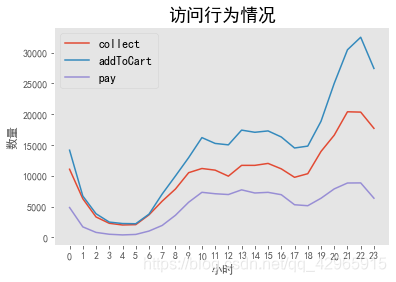
操作行为可视化
for i in pv_detatil.columns.tolist()[1:]:
    plt.plot(pv_detatil[i], label=i)
plt.legend(loc='best', fontsize=12)
plt.title('访问行为情况', fontsize=18)
plt.xticks(list(np.arange(0, 24)))
plt.xlabel('小时')
plt.ylabel('数量')
plt.grid()
plt.show()
data_user_buy = data[data.behavior_type == '4'].groupby('user_id').size()
data_user_buy.head()
user_id
100001878    36
100011562     3
100012968    15
100014060    24
100024529    26
dtype: int64
click_times = data[data.behavior_type == '1'].groupby('user_id').size()
collect_times = data[data.behavior_type == '2'].groupby('user_id').size()
addToCart_times = data[data.behavior_type == '3'].groupby('user_id').size()
pay_times = data[data.behavior_type == '4'].groupby('user_id').size()
user_behavior = pd.concat([click_times, collect_times, addToCart_times, pay_times], axis=1)
user_behavior.columns= ['click', 'collect', 'addToCart','pay']
user_behavior.fillna(0, inplace=True)
user_behavior['pay_per_click'] = round(user_behavior['click'] / user_behavior['pay'], 1)
user_behavior.head()
|
click |
collect |
addToCart |
pay |
pay_per_click |
| 100001878 |
2532 |
0.0 |
200.0 |
36.0 |
70.3 |
| 100011562 |
423 |
2.0 |
9.0 |
3.0 |
141.0 |
| 100012968 |
367 |
0.0 |
6.0 |
15.0 |
24.5 |
| 100014060 |
979 |
2.0 |
50.0 |
24.0 |
40.8 |
| 100024529 |
1121 |
1.0 |
81.0 |
26.0 |
43.1 |
user_behavior.describe()
|
click |
collect |
addToCart |
pay |
pay_per_click |
| count |
10000.000000 |
10000.000000 |
10000.000000 |
10000.000000 |
10000.000 |
| mean |
1155.058100 |
24.255600 |
34.356400 |
12.020500 |
inf |
| std |
1430.052774 |
73.900635 |
63.889429 |
19.050621 |
NaN |
| min |
1.000000 |
0.000000 |
0.000000 |
0.000000 |
2.000 |
| 25% |
297.000000 |
0.000000 |
2.000000 |
2.000000 |
51.200 |
| 50% |
703.000000 |
2.000000 |
12.000000 |
7.000000 |
101.800 |
| 75% |
1461.000000 |
18.000000 |
39.000000 |
15.000000 |
247.125 |
| max |
27720.000000 |
2935.000000 |
1810.000000 |
809.000000 |
inf |
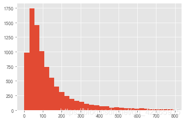
plt.hist(user_behavior[(user_behavior.pay_per_click < 800) & (user_behavior.pay_per_click >=0)].pay_per_click, bins=30)
plt.show()
# 相关性
user_behavior.corr(method='spearman').iloc[3:4, :3]
|
click |
collect |
addToCart |
| pay |
0.624926 |
0.347776 |
0.659073 |
用户消费行为分析
日ARPU和日ARPPU
# 每日活跃用户数
active_user_daily = data.groupby('date')[['user_id']].apply(lambda x: x.drop_duplicates().count())
active_user_daily.head()
|
user_id |
| date |
|
| 2014-11-18 |
6343 |
| 2014-11-19 |
6420 |
| 2014-11-20 |
6333 |
| 2014-11-21 |
6276 |
| 2014-11-22 |
6187 |
# 每日付费用户数
pay_user_daily = data[data.behavior_type == '4'].groupby('date')[['user_id']].apply(lambda x: x.drop_duplicates().count())
pay_user_daily.head()
|
user_id |
| date |
|
| 2014-11-18 |
1539 |
| 2014-11-19 |
1511 |
| 2014-11-20 |
1492 |
| 2014-11-21 |
1330 |
| 2014-11-22 |
1411 |
# 合并
consume_daily = pd.concat([active_user_daily, pay_user_daily], axis=1)
# 重新命名字段
consume_daily.columns= ['activeUserDaily', 'payUserDaily']
# 由于数据中没有给用户消费金额,设每日每位用户消费为500
consume_daily['totalIncome'] = 500
# 计算ARPU
consume_daily['ARPU'] = round(consume_daily['totalIncome'] * consume_daily['payUserDaily'] / consume_daily['activeUserDaily'], 3)
# 计算ARPPU
consume_daily['ARPPU'] = round(consume_daily['totalIncome'] * consume_daily['payUserDaily'] / consume_daily['payUserDaily'])
consume_daily.head()
|
activeUserDaily |
payUserDaily |
totalIncome |
ARPU |
ARPPU |
| date |
|
|
|
|
|
| 2014-11-18 |
6343 |
1539 |
500 |
121.315 |
500.0 |
| 2014-11-19 |
6420 |
1511 |
500 |
117.679 |
500.0 |
| 2014-11-20 |
6333 |
1492 |
500 |
117.796 |
500.0 |
| 2014-11-21 |
6276 |
1330 |
500 |
105.959 |
500.0 |
| 2014-11-22 |
6187 |
1411 |
500 |
114.029 |
500.0 |
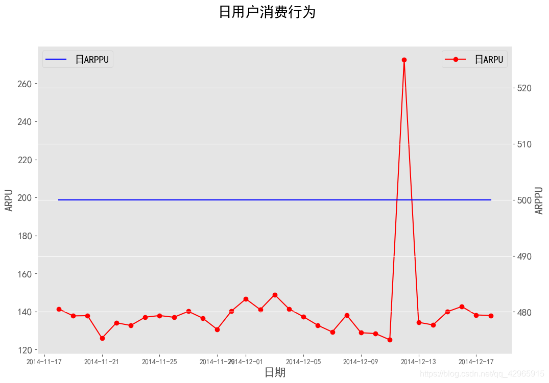
fig=plt.figure(figsize=(12, 8), dpi=100)
fig.suptitle('日用户消费行为', fontsize=20)
ax1 = fig.add_subplot(111)
ax1.plot(consume_daily['ARPU'],'ro-', label='日ARPU')
ax1.grid()
ax1.set_yticklabels(labels=list(np.arange(100, 300, 20)), fontsize=14)
ax1.set_ylabel('ARPU',fontsize=16)
ax1.legend(fontsize=14)
ax1.set_xlabel('日期', fontsize=16)
ax2 = ax1.twinx()
ax2.plot(consume_daily['ARPPU'], 'b-', label='日ARPPU')
ax2.legend(loc='upper left', fontsize=14)
ax2.set_yticklabels(labels=list(np.arange(470, 600, 10)), fontsize=14)
ax2.set_ylabel('ARPPU',fontsize=16)
fig.savefig('用户日消费行为.png', dpi=70, quality=95)
fig.show()
D:\ProgramData\Anaconda3\lib\site-packages\ipykernel_launcher.py:16: UserWarning: Matplotlib is currently using module://ipykernel.pylab.backend_inline, which is a non-GUI backend, so cannot show the figure.
  app.launch_new_instance()
用户购买次数情况分析
data['operation'] = 1
customer_operation = data.groupby(['date', 'user_id', 'behavior_type'])[['operation']].count()
customer_operation.reset_index(level=['date', 'user_id', 'behavior_type'], inplace=True)
customer_operation.head()
|
date |
user_id |
behavior_type |
operation |
| 0 |
2014-11-18 |
100001878 |
1 |
127 |
| 1 |
2014-11-18 |
100001878 |
3 |
8 |
| 2 |
2014-11-18 |
100001878 |
4 |
1 |
| 3 |
2014-11-18 |
100014060 |
1 |
23 |
| 4 |
2014-11-18 |
100014060 |
3 |
2 |
customer_operation[customer_operation.behavior_type == '4']['operation'].describe()
count    49201.000000
mean         2.443141
std          3.307288
min          1.000000
25%          1.000000
50%          1.000000
75%          3.000000
max        185.000000
Name: operation, dtype: float64
# 购买次数超过50次的用户数
customer_operation[(customer_operation.behavior_type == '4') & (customer_operation.operation > 50)].count()['user_id']
18
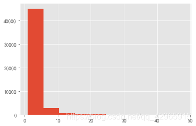
plt.hist(customer_operation[(customer_operation.behavior_type == '4') & (customer_operation.operation < 50)].operation, bins=10)
plt.show()
每天平均消费次数
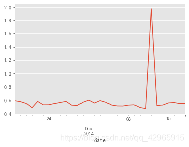
customer_operation.groupby('date').apply(lambda x: x[x.behavior_type == '4'].operation.sum() / len(x.user_id.unique())).plot()
<matplotlib.axes._subplots.AxesSubplot at 0x9e8b888>
付费率
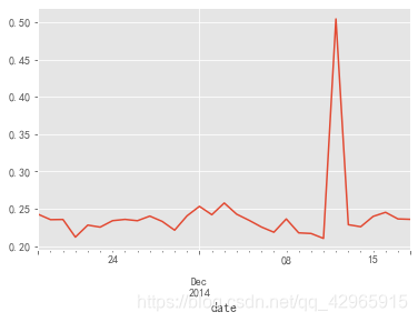
customer_operation.groupby('date').apply(lambda x: x[x.behavior_type == '4'].operation.count() / len(x.user_id.unique())).plot()
<matplotlib.axes._subplots.AxesSubplot at 0x9e77f48>
同一时间段用户消费次数分布
customer_hour_operation  = data[data.behavior_type == '4'].groupby(['user_id', 'date', 'hour',])[['operation']].sum()
customer_hour_operation.reset_index(level=['user_id', 'date', 'hour'], inplace=True)
customer_hour_operation.head()
|
user_id |
date |
hour |
operation |
| 0 |
100001878 |
2014-11-18 |
20 |
1 |
| 1 |
100001878 |
2014-11-24 |
20 |
3 |
| 2 |
100001878 |
2014-11-25 |
13 |
2 |
| 3 |
100001878 |
2014-11-26 |
16 |
2 |
| 4 |
100001878 |
2014-11-26 |
21 |
1 |
customer_hour_operation.operation.max()
97
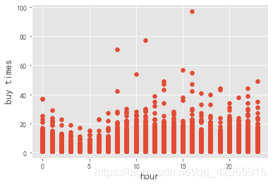
plt.scatter(customer_hour_operation.hour, customer_hour_operation.operation)
plt.xlabel('hour', fontsize=14)
plt.ylabel('buy times', fontsize=14)
plt.show()
复购行为分析
月复购率
- 按笔数(同一天超过一次)
- 按周期(同一天购买多次算一次)
# 按周期
data_rebuy = data[data.behavior_type == '4'].groupby('user_id')['date'].apply(lambda x: len(x.unique()))
data_rebuy[:5]
user_id
100001878    15
100011562     3
100012968    11
100014060    12
100024529     9
Name: date, dtype: int64
# 复购率
data_rebuy[data_rebuy >= 2].count() / data_rebuy.count()
0.8717083051991897
data_day_buy = data[data.behavior_type == '4'].groupby(['user_id']).date.apply(lambda x: x.sort_values()).diff(1).dropna().map(lambda x: x.days)
data_day_buy.head()
user_id
100001878  2439076    6
           2439090    0
           2440428    0
           2660355    1
           2672617    0
Name: date, dtype: int64
留存率
from datetime import datetime
day_user = {}
for dt in set(data.date.dt.strftime('%Y%m%d').values.tolist()):
    user = list(set(data[data.date == datetime(int(dt[:4]),int(dt[4:6]),int(dt[6:]))]['user_id'].values.tolist()))
    day_user.update({dt:user})
# 由于字典是无序的,需按日期排序
day_user = sorted(day_user.items(), key=lambda x:x[0], reverse=False)
# 计算每日新增用户
a = {}
t = set(day_user[0][1])
a.update({'20141118':t})
for i in day_user[1:]:
    j = (set(i[1]) - t)
    a.update({i[0]:j})
    t = t | set(i[1])
# 目的是为了和day_user类型一样
a = sorted(a.items(), key=lambda x:x[0], reverse=False)
# 计算留存
retention = {}
ls = []
for i, k in enumerate(a):
    ls.append(len(k[1]))
    for j in day_user[i+1:]:
        li = len(set(k[1]) & set(j[1]))
        ls.append(li)
    retention.update({k[0]: ls})
    ls = []
# 目的是为了和day_user类型一样
retention = sorted(retention.items(), key=lambda x:x[0], reverse=False)
re = {}
for i in retention[:16]:
    re.update({i[0]: i[1][:15]})
retention = pd.DataFrame(re)
retention =  retention.T
retention.drop([8,9,11,12,13], axis=1, inplace=True)
retention.columns = ['新增用户', '次日留存', '2日留存','3日留存', '4日留存','5日留存', '6日留存', '7日留存', '10日留存','14日留存']
div = retention.columns.tolist()[:-1]
for i, dived in enumerate(retention.columns.tolist()[1:]):
    retention['{}率'.format(dived)] = round(retention[dived] / retention['新增用户'], 3)
cols=['新增用户','次日留存','次日留存率','2日留存','2日留存率','3日留存','3日留存率','4日留存','4日留存率','5日留存','5日留存率','6日留存','6日留存率','7日留存','7日留存率','10日留存','10日留存率','14日留存','14日留存率']
retention = retention[cols]
retention.sort_index(inplace=True)
retention.head()
|
新增用户 |
次日留存 |
次日留存率 |
2日留存 |
2日留存率 |
3日留存 |
3日留存率 |
4日留存 |
4日留存率 |
5日留存 |
5日留存率 |
6日留存 |
6日留存率 |
7日留存 |
7日留存率 |
10日留存 |
10日留存率 |
14日留存 |
14日留存率 |
| 20141118 |
6343 |
5137 |
0.810 |
5000 |
0.788 |
4861 |
0.766 |
4763 |
0.751 |
4810 |
0.758 |
4916 |
0.775 |
4792 |
0.755 |
4627 |
0.729 |
4806 |
0.758 |
| 20141119 |
1283 |
783 |
0.610 |
770 |
0.600 |
736 |
0.574 |
769 |
0.599 |
777 |
0.606 |
758 |
0.591 |
746 |
0.581 |
709 |
0.553 |
757 |
0.590 |
| 20141120 |
550 |
305 |
0.555 |
274 |
0.498 |
298 |
0.542 |
295 |
0.536 |
286 |
0.520 |
299 |
0.544 |
306 |
0.556 |
310 |
0.564 |
290 |
0.527 |
| 20141121 |
340 |
164 |
0.482 |
176 |
0.518 |
178 |
0.524 |
158 |
0.465 |
172 |
0.506 |
174 |
0.512 |
160 |
0.471 |
182 |
0.535 |
170 |
0.500 |
| 20141122 |
250 |
122 |
0.488 |
110 |
0.440 |
95 |
0.380 |
93 |
0.372 |
105 |
0.420 |
105 |
0.420 |
106 |
0.424 |
113 |
0.452 |
123 |
0.492 |
retention.index.str[-4:]
Index(['1118', '1119', '1120', '1121', '1122', '1123', '1124', '1125', '1126',
       '1127', '1128', '1129', '1130', '1201', '1202', '1203'],
      dtype='object')
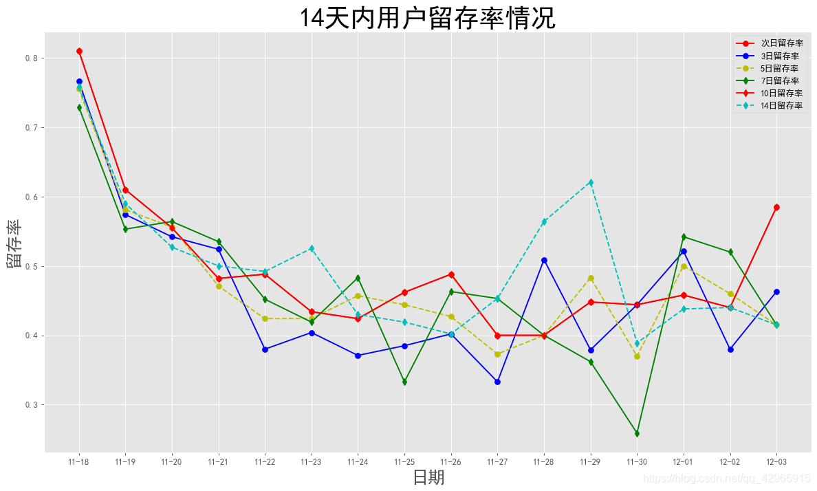
plt.figure(figsize=(16, 9), dpi=90)
x = [i[:2] + '-' + i[2:] for i in retention.index.str[-4:].tolist()]
y1 = retention['次日留存率']
y2 = retention['3日留存率']
y3 = retention['7日留存率']
y4 = retention['10日留存率']
y5 = retention['14日留存率']

plt.plot(x, y1, 'ro-', label='次日留存率')
plt.plot(x, y2, 'bo-', label='3日留存率')
plt.plot(x, y3, 'yo--', label='5日留存率')
plt.plot(x, y4, 'gd-', label='7日留存率')
plt.plot(x, y1, 'rd-', label='10日留存率')
plt.plot(x, y5, 'cd--', label='14日留存率')

plt.legend(loc='best')
plt.title('14天内用户留存率情况', fontsize=30)
plt.xlabel('日期', fontsize=20)
plt.ylabel('留存率', fontsize=20)
plt.show()
漏斗流失分析
data_user_count = data.groupby('behavior_type').size()
data_user_count
behavior_type
1    11550581
2      242556
3      343564
4      120205
dtype: int64
pv_all = data.user_id.count()
pv_all
12256906
pv_click = (pv_all - data_user_count[0]) / pv_all
click_cart = 1 - (data_user_count[0] - data_user_count[2]) / data_user_count[0]
cart_collect = 1 - (data_user_count[2] - data_user_count[1]) / data_user_count[2]
collect_pay = 1 - (data_user_count[1] - data_user_count[3]) / data_user_count[1]
cart_pay = 1 - (data_user_count[2] - data_user_count[3]) / data_user_count[2]
change_rate = pd.DataFrame({'计数': [pv_all, data_user_count[0], data_user_count[2], data_user_count[3]],\
                            '单一转化率':[1, pv_click, click_cart, cart_pay]}, index=['浏览', '点击', '加入购物车', '支付'])
change_rate['总体转化率'] = change_rate['计数'] / pv_all
change_rate
|
计数 |
单一转化率 |
总体转化率 |
| 浏览 |
12256906 |
1.000000 |
1.000000 |
| 点击 |
11550581 |
0.057627 |
0.942373 |
| 加入购物车 |
343564 |
0.029744 |
0.028030 |
| 支付 |
120205 |
0.349877 |
0.009807 |
二八理论分析淘宝商品
goods_category = data[data.behavior_type == '4'].groupby('item_category')[['user_id']].count().rename(columns={'user_id':'购买量'}).sort_values(by='购买量', ascending=False)
goods_category['累计购买量'] = goods_category.cumsum()
goods_category['占比'] = goods_category['累计购买量'] / goods_category['购买量'].sum()
goods_category['分类'] = np.where(goods_category['占比'] <= 0.80, '产值前80%', '产值后20%')
goods_pareto = goods_category.groupby('分类')[['购买量']].count().rename(columns={'购买量':'商品数'})
goods_pareto['商品数占比'] = round(goods_pareto['商品数'] / goods_pareto['商品数'].sum(), 3)
goods_pareto
|
商品数 |
商品数占比 |
| 分类 |
|
|
| 产值前80% |
726 |
0.156 |
| 产值后20% |
3939 |
0.844 |
用户细分(RFM)
计算R
from datetime import datetime
recent_user_buy = data[data.behavior_type == '4'].groupby('user_id')['date'].apply(lambda x: datetime(2014, 12, 20)-x.sort_values().iloc[-1])
recent_user_buy = recent_user_buy.reset_index()
recent_user_buy.columns = ['user_id', 'recent']
recent_user_buy.recent = recent_user_buy.recent.map(lambda x: x.days)
recent_user_buy.head()
|
user_id |
recent |
| 0 |
100001878 |
2 |
| 1 |
100011562 |
4 |
| 2 |
100012968 |
2 |
| 3 |
100014060 |
2 |
| 4 |
100024529 |
4 |
计算F
buy_freq = data[data.behavior_type == '4'].groupby('user_id').date.count()
buy_freq = buy_freq.reset_index().rename(columns={'date': 'freq'})
buy_freq.head()
|
user_id |
freq |
| 0 |
100001878 |
36 |
| 1 |
100011562 |
3 |
| 2 |
100012968 |
15 |
| 3 |
100014060 |
24 |
| 4 |
100024529 |
26 |
rfm = pd.merge(recent_user_buy, buy_freq, right_on='user_id', left_on='user_id')
rfm.head()
|
user_id |
recent |
freq |
| 0 |
100001878 |
2 |
36 |
| 1 |
100011562 |
4 |
3 |
| 2 |
100012968 |
2 |
15 |
| 3 |
100014060 |
2 |
24 |
| 4 |
100024529 |
4 |
26 |
给予指标
rfm['R_value'] = pd.qcut(rfm.recent, 2, labels=['高', '低'])
rfm['F_value'] = pd.qcut(rfm.freq, 2, labels=['低', '高'])
rfm['rf'] = rfm['R_value'].str.cat(rfm.F_value)
rfm.head()
|
user_id |
recent |
freq |
R_value |
F_value |
rf |
| 0 |
100001878 |
2 |
36 |
高 |
高 |
高高 |
| 1 |
100011562 |
4 |
3 |
高 |
低 |
高低 |
| 2 |
100012968 |
2 |
15 |
高 |
高 |
高高 |
| 3 |
100014060 |
2 |
24 |
高 |
高 |
高高 |
| 4 |
100024529 |
4 |
26 |
高 |
高 |
高高 |
用户分类
def trans_value(x):
    if x == '高高': return '价值用户'
    elif x == '高低': return '发展用户'
    elif x == '低高': return '挽留客户'
    else: return '潜在客户'
rfm['rank'] = rfm.rf.apply(trans_value)
rfm.head()
|
user_id |
recent |
freq |
R_value |
F_value |
rf |
rank |
| 0 |
100001878 |
2 |
36 |
高 |
高 |
高高 |
价值用户 |
| 1 |
100011562 |
4 |
3 |
高 |
低 |
高低 |
发展用户 |
| 2 |
100012968 |
2 |
15 |
高 |
高 |
高高 |
价值用户 |
| 3 |
100014060 |
2 |
24 |
高 |
高 |
高高 |
价值用户 |
| 4 |
100024529 |
4 |
26 |
高 |
高 |
高高 |
价值用户 |
统计不同类型用户结果及可视化
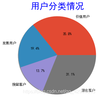
rfm.groupby('rank')[['user_id']].count()
|
user_id |
| rank |
|
| 价值用户 |
3179 |
| 发展用户 |
1721 |
| 挽留客户 |
1219 |
| 潜在客户 |
2767 |
plt.pie(rfm.groupby('rank')[['user_id']].count().values.tolist(), labels=rfm.groupby('rank')[['user_id']].count().index.tolist(), shadow=True, autopct='%.1f%%', radius=1.5, textprops=dict(fontsize=12))
plt.title('用户分类情况', fontsize=30, pad=45, color='blue')
plt.show()
D:\ProgramData\Anaconda3\lib\site-packages\ipykernel_launcher.py:1: MatplotlibDeprecationWarning: Non-1D inputs to pie() are currently squeeze()d, but this behavior is deprecated since 3.1 and will be removed in 3.3; pass a 1D array instead.
  """Entry point for launching an IPython kernel.
结论与建议
- 这一月内的日访问量和日访问用户数呈现相同趋势,日访问量大都在35万-40万之间波动,日访客数大都在6200-6600波动,
在双十二购物狂欢节期间出现了剧增。
- 根据每小时用户访问行为可以看出用户主要访问淘宝的时间段是在白天10点以后,晚上9点左右达到访客人数的峰值
- 由于没有用户消费金额,无法得出日ARPU与日ARPPU具体情况,但是可以肯定的是日ARPPU是高于日ARPU的。
- 用户日平均消费次数在0.5次左右波动。
- 付费率是在20%-25%之间波动,在双十二期间达到50%
- 淘宝用户一天中每小时的消费次数主要在30次以内。
- 用户复购率为87%
- 可以看出,在点击商品到加入购物车的转化率大约为3%,而从购物车到支付大约35%,因此淘宝应该优化商品界面以及对商品相关的优化,使点击商品到加入购物车的转化率提高。
- 可以看出16%的商品占了80%的商品购买量,84%的商品仅提供了20%的商品购买量,因此应对后84%的商品进行优化、撤销等操作来提高后80%商品的购买量。
- 淘宝留存率虽然会在短期内从80%下滑到40%,但最终会在40%左右波动,留存率较好。3/5/7/10日留存率差异不大,14日留存率均高于40%。