问题描述
考虑代价函数
f
i
(
x
i
,
t
)
=
∥
x
i
−
x
i
∗
(
t
)
∥
2
.
f_i(x_i,t)=\|x_i-x_i^*(t)\|^2.
fi(xi,t)=∥xi−xi∗(t)∥2.
求解一个简单的优化问题实例:
min
1
2
∑
i
=
1
n
f
i
(
x
i
,
t
)
s.t.
f
i
(
x
i
,
t
)
≤
1
x
i
−
x
j
=
0
\begin{aligned} \min &\quad \frac{1}{2}\sum_{i=1}^n f_i(x_i,t)\\ \operatorname{s.t.} &\quad f_i(x_i,t)\leq 1\\ &\quad x_i-x_j=0 \end{aligned}
mins.t.21i=1∑nfi(xi,t)fi(xi,t)≤1xi−xj=0
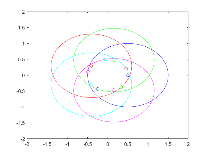
如下图所示,参考位置
x
i
∗
(
t
)
x_i^*(t)
xi∗(t)由菱形表示,初始位置
x
i
(
0
)
x_i(0)
xi(0)由小圆圈表示,不等式约束
f
i
(
x
i
,
t
)
≤
1
f_i(x_i,t)\leq 1
fi(xi,t)≤1由大圆圈表示。
内点法
设计barrier构建带惩罚项的代价函数
L
i
(
x
,
t
)
=
f
i
(
x
,
t
)
−
1
ρ
(
t
)
log
(
1
−
ρ
(
t
)
(
f
i
(
x
i
,
t
)
−
1
)
)
,
ρ
(
t
)
=
a
1
e
a
2
t
,
a
1
,
a
2
>
0
,
L_i(x,t) = f_i(x,t)-\frac{1}{\rho(t)}\log(1-\rho(t)(f_i(x_i,t)-1)),\quad \rho(t)=a_1e^{a_2t},\quad a_1,a_2>0,
Li(x,t)=fi(x,t)−ρ(t)1log(1−ρ(t)(fi(xi,t)−1)),ρ(t)=a1ea2t,a1,a2>0,
其中,梯度、Hessian和关于时间的变化率为
∇
L
i
(
x
i
,
t
)
=
∇
f
i
(
x
i
,
t
)
+
∇
f
i
(
x
i
,
t
)
1
−
ρ
(
t
)
(
f
i
(
x
i
,
t
)
−
1
)
∂
∂
t
∇
L
i
(
x
i
,
t
)
=
∂
∂
t
∇
f
i
(
x
i
,
t
)
+
∂
∇
f
i
(
x
i
,
t
)
/
∂
t
1
−
ρ
(
t
)
(
f
i
(
x
i
,
t
)
−
1
)
+
(
ρ
˙
(
t
)
(
f
i
(
x
i
,
t
)
−
1
)
+
ρ
(
t
)
∂
f
i
(
x
i
,
t
)
/
∂
t
)
∇
f
i
(
x
i
,
t
)
(
1
−
ρ
(
t
)
(
f
i
(
x
i
,
t
)
−
1
)
)
2
∇
2
L
i
(
x
i
,
t
)
=
∇
2
f
i
(
x
i
,
t
)
+
∇
2
f
i
(
x
i
,
t
)
1
−
ρ
(
t
)
(
f
i
(
x
i
,
t
)
−
1
)
+
ρ
(
t
)
∇
f
i
(
x
i
,
t
)
∇
f
i
(
x
i
,
t
)
T
1
−
ρ
(
t
)
(
f
i
(
x
i
,
t
)
−
1
)
\begin{aligned} \nabla L_i(x_i,t)&=\nabla f_i(x_i,t)+\frac{\nabla f_i(x_i,t)}{1-\rho(t)(f_i(x_i,t)-1)}\\ \frac{\partial}{\partial t}\nabla L_i(x_i,t)&=\frac{\partial}{\partial t}\nabla f_i(x_i,t)+\frac{\partial\nabla f_i(x_i,t)/\partial t}{1-\rho(t)(f_i(x_i,t)-1)}\\ &\quad+\frac{(\dot \rho(t)(f_i(x_i,t)-1)+\rho(t)\partial f_i(x_i,t)/\partial t)\nabla f_i(x_i,t)}{(1-\rho(t)(f_i(x_i,t)-1))^2}\\ \nabla^2 L_i(x_i,t)&=\nabla^2 f_i(x_i,t)+\frac{\nabla^2 f_i(x_i,t)}{1-\rho(t)(f_i(x_i,t)-1)}+\frac{\rho(t)\nabla f_i(x_i,t)\nabla f_i(x_i,t)^T}{1-\rho(t)(f_i(x_i,t)-1)} \end{aligned}
∇Li(xi,t)∂t∂∇Li(xi,t)∇2Li(xi,t)=∇fi(xi,t)+1−ρ(t)(fi(xi,t)−1)∇fi(xi,t)=∂t∂∇fi(xi,t)+1−ρ(t)(fi(xi,t)−1)∂∇fi(xi,t)/∂t+(1−ρ(t)(fi(xi,t)−1))2(ρ˙(t)(fi(xi,t)−1)+ρ(t)∂fi(xi,t)/∂t)∇fi(xi,t)=∇2fi(xi,t)+1−ρ(t)(fi(xi,t)−1)∇2fi(xi,t)+1−ρ(t)(fi(xi,t)−1)ρ(t)∇fi(xi,t)∇fi(xi,t)T
参考Sun 20201,设计如下控制律
u
i
=
−
β
(
∇
2
L
i
(
x
i
,
t
)
)
−
1
∑
j
∈
N
i
sgn
(
x
i
−
x
j
)
+
ϕ
i
(
t
)
ϕ
i
(
t
)
=
−
(
∇
2
L
i
(
x
i
,
t
)
)
−
1
(
∇
L
i
(
x
i
,
t
)
+
∂
∂
t
∇
L
i
(
x
i
,
t
)
)
\begin{aligned} u_i&=-\beta(\nabla^2L_i(x_i,t))^{-1}\sum_{j\in\mathcal N_i}\operatorname{sgn}(x_i-x_j)+\phi_i(t)\\ \phi_i(t)&=-(\nabla^2L_i(x_i,t))^{-1}\left(\nabla L_i(x_i,t)+\frac{\partial}{\partial t}\nabla L_i(x_i,t) \right) \end{aligned}
uiϕi(t)=−β(∇2Li(xi,t))−1j∈Ni∑sgn(xi−xj)+ϕi(t)=−(∇2Li(xi,t))−1(∇Li(xi,t)+∂t∂∇Li(xi,t))
MATLAB实现
下面给出MATLAB仿真结果和源代码。
仿真结果
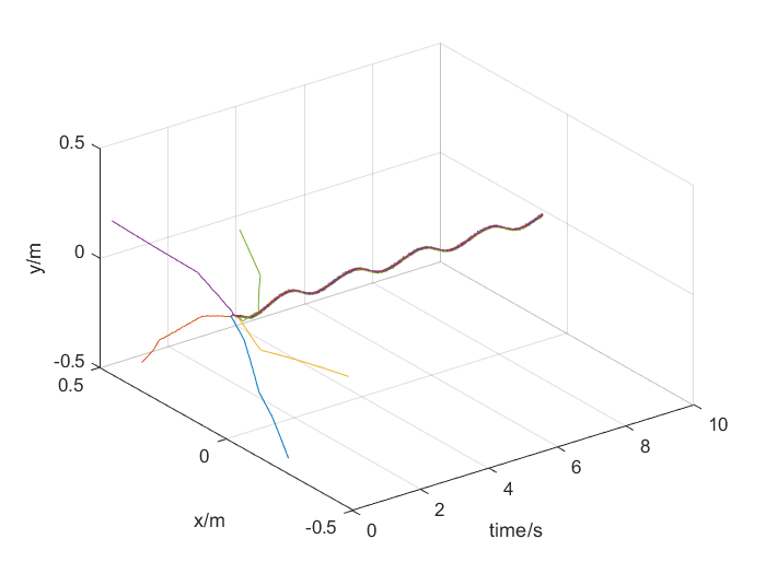
仿真结果动图如下所示。
每一个
x
i
x_i
xi的轨迹如下图所示,可以看出所有agent的状态一致且收敛到优化问题的解。
源代码
robot_num = 5;

% reference
angle_central = 2*pi/robot_num;
if ~mod(robot_num,2)
    pos_ref = [cos([0 kron(1:(robot_num-1)/2,[1,-1]) robot_num/2]*angle_central)',...
        sin([0 kron(1:(robot_num-1)/2,[1,-1]) robot_num/2]*angle_central)']/2;
else
    pos_ref = [cos([0 kron(1:(robot_num-1)/2,[1,-1])]*angle_central)',...
        sin([0 kron(1:(robot_num-1)/2,[1,-1])]*angle_central)']/2;
end

% topology
graph = selectTopology(robot_num,pos_ref);

% initial position
pos_rob = pos_ref*rot2(2*pi/3);

% initial control
u_rob = zeros(size(pos_rob));

% reference control
u_ref_func = @(t) pos_ref./normby(pos_ref,1)*sin(pi*t)/2.*(-1).^(0:robot_num-1)';
u_ref = u_ref_func(0);

% plot
color_list = ['b','g','m','r','c'];
for i=1:robot_num
    hg_pos_rob(i) = plot(pos_rob(i,1),pos_rob(i,2),[color_list(i) 'o']); hold on
    pos_circ = circle_(pos_ref(i,:),1);
    hg_pos_circ(i) = plot(pos_circ(:,1),pos_circ(:,2),color_list(i));
    hg_pos_ref(i) = plot(pos_ref(i,1),pos_ref(i,2),[color_list(i) 'd']);
    hg_u_ref(i) = quiver(pos_ref(i,1),pos_ref(i,2),u_ref(i,1),u_ref(i,2),'color',color_list(i),'LineStyle', '--');
    axis([-2 2 -2 2])
end
hold off

% functions
a1 = 1; a2 = 1; rho = a1*exp(a2*0); cost_hessian = 2*eye(2);
cost_ref = @(i,pos_rob,pos_ref) (pos_rob(i,:)-pos_ref(i,:))*(pos_rob(i,:)-pos_ref(i,:))';
cost_ref_dot = @(i,pos_rob,u_ref) -2*(pos_rob(i,:)-pos_ref(i,:))*u_ref(i,:)';
cost_ref_nabla = @(i,pos_rob,pos_ref) 2*(pos_rob(i,:)-pos_ref(i,:))';
cost_ref_nabla_dot = @(i,u_ref) -2*u_ref(i,:)';
cost_penalty = @(i,pos_rob,rho) cost_ref(i,pos_rob,pos_ref)-(1/rho)*log(1-rho*(cost_ref(i,pos_rob,pos_ref)-1));
cost_penalty_nabla = @(i,pos_rob,pos_ref,rho) cost_ref_nabla(i,pos_rob,pos_ref)*(1+1/(1-rho*(cost_ref(i,pos_rob,pos_ref)-1)));
cost_penalty_nabla_dot = @(i,pos_rob,pos_ref,rho) cost_ref_nabla_dot(i,u_ref)*(1+1/(1-rho*(cost_ref(i,pos_rob,pos_ref)-1)))+...
    rho*(a2*(cost_ref(i,pos_rob,pos_ref)-1)+cost_ref_dot(i,pos_rob,u_ref))/(1-rho*(cost_ref(i,pos_rob,pos_ref)-1))^2;
cost_penalty_hessian = @(i,pos_rob,pos_ref,rho) cost_hessian*(1+1/(1-rho*(cost_ref(i,pos_rob,pos_ref)-1)))+...
    rho*cost_ref_nabla(i,pos_rob,pos_ref)*cost_ref_nabla(i,pos_rob,pos_ref)'/(1-rho*(cost_ref(i,pos_rob,pos_ref)-1));
% test error
cost_ref(i,pos_rob,pos_ref);
cost_ref_dot(i,pos_rob,u_ref);
cost_ref_nabla(i,pos_rob,pos_ref);
cost_ref_nabla_dot(i,u_ref);
cost_penalty(i,pos_rob,rho);
cost_penalty_nabla(i,pos_rob,pos_ref,rho);
cost_penalty_nabla_dot(i,pos_rob,pos_ref,rho);
cost_penalty_hessian(i,pos_rob,pos_ref,rho);
disp('All functions are correct.');

% simulation
pos_data = pos_rob;
dt = 0.005;
T = 10;
loop = 0;
playspeed = 4;
video_on = true;
for t=0:dt:T
    loop = loop+1;
    % control
    u_ref = u_ref_func(t);
    beta = 1; hessian_inv = []; u_rob_tp = u_rob';
    for i=1:robot_num
       phi(:,i) = -cost_penalty_hessian(i,pos_rob,pos_ref,rho)^-1*...
           (cost_penalty_nabla(i,pos_rob,pos_ref,rho)+cost_penalty_nabla_dot(i,pos_rob,pos_ref,rho));
       hessian_inv = blkdiag(hessian_inv,cost_penalty_hessian(i,pos_rob,pos_ref,rho)^-1);
    end
    sign_rob = (graph.incidence*sign(graph.incidence'*pos_rob))';
    u_rob_tp(:) = -beta*hessian_inv*sign_rob(:)+phi(:);
    u_rob = u_rob_tp';
    % update
    pos_ref = pos_ref+dt*u_ref;
    pos_rob = pos_rob+dt*u_rob;
    pos_data(:,:,loop) = pos_rob;
    % plot
    for i=1:robot_num
        set(hg_pos_rob(i),'xdata',pos_rob(i,1),'ydata',pos_rob(i,2));
        pos_circ = circle_(pos_ref(i,:),1);
        set(hg_pos_circ(i),'xdata',pos_circ(:,1),'ydata',pos_circ(:,2));
        set(hg_pos_ref(i),'xdata',pos_ref(i,1),'ydata',pos_ref(i,2));
        set(hg_u_ref(i),'xdata',pos_ref(i,1),'ydata',pos_ref(i,2),...
            'udata',u_ref(i,1),'vdata',u_ref(i,2));
        axis([-2 2 -2 2])
    end
    % video
    if mod(loop,playspeed)==0&&video_on
        frame(loop/playspeed) = getframe(gcf);
    end
    drawnow
end

% write video
if video_on
    savevideo('video',frame);
end

% result
figure
t_data = 0:dt:T;
xpos_data = squeeze(pos_data(:,1,:));
ypos_data = squeeze(pos_data(:,2,:));
plot3(kron(ones(robot_num,1),t_data)',xpos_data',ypos_data');
xlabel('time/s');ylabel('x/m');zlabel('y/m');grid
源代码我已上传至我的GitHub,见项目paper-simulation。运行Sun2020Distributed文件夹下的文件time_varying_optimization.m,即可得到上面的仿真结果。代码中部分函数用到了RTB,下载和安装说明点击这里。
如果喜欢,欢迎点赞和fork。
-
Sun, S., & Ren, W. (2020). Distributed Continuous-Time Optimization with Time-Varying Objective Functions and Inequality Constraints. Retrieved from http://arxiv.org/abs/2009.02378