sklearn专题六：聚类算法K-Means

2023-05-16

1 概述

1.1 无监督学习与聚类算法

1.2 sklearn中的聚类算法

2 KMeans

2.1 KMeans是如何工作的

2.2 簇内误差平方和的定义和解惑

2.3 KMeans算法的时间复杂度

3 sklearn.cluster.KMeans

3.1 重要参数n_clusters

3.1.1 先进行一次聚类看看吧

3.1.2 聚类算法的模型评估指标

3.1.2.1 当真实标签已知的时候

3.1.2.2 当真实标签未知的时候：轮廓系数

3.1.2.3 当真实标签未知的时候：Calinski-Harabaz Index

3.1.3 案例：基于轮廓系数来选择n_clusters

3.3 重要参数max_iter & tol：让迭代停下来

3.4 重要属性与重要接口

3.5 函数cluster.k_means

4 案例：聚类算法用于降维，KMeans的矢量量化应用

1 概述

1.1 无监督学习与聚类算法

在过去的五周之内，我们学习了决策树，随机森林，逻辑回归，他们虽然有着不同的功能，但却都属于 “有监督学习 ” 的一部分，即是说，模型在训练的时候，即需要特征矩阵 X ，也需要真实标签 y。机器学习当中，还有相当一部分算法属于 “ 无监督学习 ” ，无监督的算法在训练的时候只需要特征矩阵 X ，不需要标签。我们曾经学过的 PCA降维算法就是无监督学习中的一种，聚类算法，也是无监督学习的代表算法之一。

聚类算法又叫做 “无监督分类”，其目的是将数据划分成有意义或有用的组（或簇）。这种划分可以基于我们的业务需求或建模需求来完成，也可以单纯地帮助我们探索数据的自然结构和分布。比如在商业中，如果我们手头有大量的当前和潜在客户的信息，我们可以使用聚类将客户划分为若干组，以便进一步分析和开展营销活动，最有名的客户价值判断模型 RFM ，就常常和聚类分析共同使用。再比如，聚类可以用于降维和矢量量化（vector quantization），可以将高维特征压缩到一列当中，常常用于图像，声音，视频等非结构化数据，可以大幅度压缩数据量。

聚类 vs 分类

1.2 sklearn中的聚类算法

聚类算法在 sklearn中有两种表现形式，一种是类（和我们目前为止学过的分类算法以及数据预处理方法们都一样），需要实例化，训练并使用接口和属性来调用结果。另一种是函数( function)，只需要输入特征矩阵和超参数，即可返回聚类的结果和各种指标。

输入数据

需要注意的一件重要事情是，该模块中实现的算法可以采用不同类型的矩阵作为输入。所有方法都接受形状[n_samples ， n_features] 的标准特征矩阵，这些可以从 sklearn.feature_extraction模块中的类中获得。对于亲和力传播，光谱聚类和 DBSCAN ，还可以输入形状 [n_samples ， n_samples]的相似性矩阵，我们可以使用sklearn.metrics.pairwise 模块中的函数来获取相似性矩阵。

2 KMeans

2.1 KMeans是如何工作的

作为聚类算法的典型代表， KMeans 可以说是最简单的聚类算法没有之一，那它是怎么完成聚类的呢？

在 KMeans 算法中，簇的个数 K 是一个超参数，需要我们人为输入来确定。 KMeans的核心任务就是根据我们设定好的 K ，找出 K个最优的质心，并将离这些质心最近的数据分别分配到这些质心代表的簇中去。具体过程可以总结如下：

那什么情况下，质心的位置会不再变化呢？当我们找到一个质心，在每次迭代中被分配到这个质心上的样本都是一致的，即每次新生成的簇都是一致的，所有的样本点都不会再从一个簇转移到另一个簇，质心就不会变化了。

这个过程在可以由下图来显示，我们规定，将数据分为 4 簇（ K=4 ），其中白色 X 代表质心的位置：

在数据集下多次迭代(iteration)，就会有：

可以看见，第六次迭代之后，基本上质心的位置就不再改变了，生成的簇也变得稳定。此时我们的聚类就完成了，我们可以明显看出， KMeans 按照数据的分布，将数据聚集成了我们规定的 4类，接下来我们就可以按照我们的业务需求或者算法需求，对这四类数据进行不同的处理。

2.2 簇内误差平方和的定义和解惑

聚类算法聚出的类有什么含义呢？这些类有什么样的性质？我们认为， 被分在同一个簇中的数据是有相似性的，而 不同簇中的数据是不同的，当聚类完毕之后，我们就要分别去研究每个簇中的样本都有什么样的性质，从而根据业务需求制定不同的商业或者科技策略。这个听上去和我们在上周的评分卡案例中讲解的 “ 分箱”概念有些类似，即我们分箱的目的是希望，一个箱内的人有着相似的信用风险，而不同箱的人的信用风险差异巨大，以此来区别不同信用度的人，因此我们追求 “ 组内差异小，组间差异大 ” 。聚类算法也是同样的目的，我们追求 “簇内差异小，簇外差异大 ” 。而这个 “ 差异 “ ，由 样本点到其所在簇的质心的距离 来衡量。

对于一个簇来说，所有样本点到质心的距离之和越小，我们就认为这个簇中的样本越相似，簇内差异就越小。而距离的衡量方法有多种，令表示簇中的一个样本点，表示该簇中的质心， n 表示每个样本点中的特征数目， i表示组成点的每个特征，则该样本点到质心的距离可以由以下距离来度量：

如我们采用欧几里得距离，则一个簇中所有样本点到质心的距离的平方和为：

其中， m 为一个簇中样本的个数， j 是每个样本的编号。这个公式被称为 簇内平方和 （ cluster Sum of Square），又叫做 Inertia 。而将一个数据集中的所有簇的簇内平方和相加，就得到了整体平方和（Total Cluster Sum of Square ），又叫做 total inertia 。 Total Inertia 越小，代表着每个簇内样本越相似，聚类的效果就越好。因此 KMeans 追求的是，求解能够让 Inertia 最小化的质心。实际上，在质心不断变化不断迭代的过程中，总体平方和是越来越小的。我们可以使用数学来证明，当整体平方和最小的时候，质心就不再发生变化了。如此， K-Means的求解过程，就变成了一个最优化问题。

这是我们在这个课程中第二次遇见最优化问题，即需要将某个指标最小化来求解模型中的一部分信息。记得我们在逻辑回归中式怎么做的吗？我们在一个固定的方程 $y(x)=\frac{1}{1+e^{\theta^{T_{x}}}}$ 中最小化损失函数来求解模型的参数向量，并且基于参数向量的存在去使用模型。而在 KMeans 中，我们在一个固定的簇数K下，最小化总体平方和来求解最佳质心，并基于质心的存在去进行聚类。两个过程十分相似，并且，整体距离平方和的最小值其实可以使用梯度下降来求解。因此，有许多博客和教材都这样写道：簇内平方和 / 整体平方和是 KMeans 的损失函数。

解惑： Kmeans 有损失函数吗？

记得我们在逻辑回归中曾有这样的结论：损失函数本质是用来衡量模型的拟合效果的，只有有着求解参数需求的算法，才会有损失函数。 Kmeans不求解什么参数，它的模型本质也没有在拟合数据，而是在对数据进行一种探索。所以如果你去问大多数数据挖掘工程师，甚至是算法工程师，他们可能会告诉你说， K-Means不存在什么损失函数， Inertia 更像是 Kmeans 的模型评估指标，而非损失函数。

但我们类比过了 Kmeans 中的 Inertia和逻辑回归中的损失函数的功能，我们发现它们确实非常相似。所以，从 “ 求解模型中的某种信息，用于后续模型的使用 “ 这样的功能来看，我们可以认为 Inertia 是 Kmeans中的损失函数，虽然这种说法并不严谨。

对比来看，在决策树中，我们有衡量分类效果的指标准确度accuracy，准确度所对应的损失叫做泛化误差，但我们不能通过最小化泛化误差来求解某个模型中需要的信息，我们只是希望模型的效果上表现出来的泛化误差很小。因此决策树， KNN 等算法，是绝对没有损失函数的。

大家可以发现，我们的 Inertia是基于欧几里得距离的计算公式得来的。实际上，我们也可以使用其他距离，每个距离都有自己对应的 Inertia 。在过去的经验中，我们总结出不同距离所对应的质心选择方法和 Inertia ，在Kmeans中，只要使用了正确的质心和距离组合，无论使用什么样的距离，都可以达到不错的聚类效果：

而这些组合，都可以由严格的数学证明来推导。在 sklearn当中，我们无法选择使用的距离，只能使用欧式距离。因此，我们也无需去担忧这些距离所搭配的质心选择是如何得来的了。

2.3 KMeans算法的时间复杂度

除了模型本身的效果之外，我们还使用另一种角度来度量算法：算法复杂度。算法的复杂度分为时间复杂度和空间复杂度，时间复杂度是指执行算法所需要的计算工作量，常用大O符号表述；而空间复杂度是指执行这个算法所需要的内存空间。如果一个算法的效果很好，但需要的时间复杂度和空间复杂度都很大，那我们将会权衡算法的效果和所需的计算成本之间，比如我们在降维算法和特征工程那两章中，我们尝试了一个很大的数据集下 KNN和随机森林所需的运行时间，以此来表明我们降维的目的和决心。

和 KNN 一样， KMeans 算法是一个计算成本很大的算法。在这里，我们介绍 KMeans算法的时间和空间复杂度来加深对 KMeans 的理解。

KMeans 算法的平均复杂度是 O(k*n*T) ，其中 k 是我们的超参数，所需要输入的簇数， n是整个数据集中的样本量，T 是所需要的迭代次数（相对的， KNN 的平均复杂度是 O(n) ）。在最坏的情况下， KMeans的复杂度可以写作 $O(n^{(k+2)/p})$ ，其中 n 是整个数据集中的样本量， p 是特征总数。这个最高复杂度是由 D. Arthur 和 S. Vassilvitskii在2006 年发表的论文 ”k-means 方法有多慢？ “ 中提出的。

在实践中，比起其他聚类算法， k-means 算法已经快了，但它一般找到 Inertia的局部最小值。这就是为什么多次重启它会很有用。

3 sklearn.cluster.KMeans

class sklearn.cluster.KMeans ( n_clusters=8 , init=’k-means++’ , n_init=10 , max_iter=300 , tol=0.0001,precompute_distances=’auto’ , verbose=0 , random_state=None , copy_x=True , n_jobs=None , algorithm=’auto’ )

3.1 重要参数n_clusters

n_clusters 是 KMeans 中的 k ，表示着我们告诉模型我们要分几类。这是 KMeans 当中唯一一个必填的参数，默认为8类，但通常我们的聚类结果会是一个小于 8 的结果。通常，在开始聚类之前，我们并不知道 n_clusters究竟是多少，因此我们要对它进行探索。

3.1.1 先进行一次聚类看看吧

当我们拿到一个数据集，如果可能的话，我们希望能够通过绘图先观察一下这个数据集的数据分布，以此来为我们聚类时输入的 n_clusters 做一个参考。

首先，我们来自己创建一个数据集。这样的数据集是我们自己创建，所以是有标签的。

from sklearn.datasets import make_blobs
import matplotlib.pyplot as plt

#自己创建数据集
# n_samples:表示数据样本点个数,默认值100
# n_features:是每个样本的特征（或属性）数，也表示数据的维度，默认值是2
# centers:表示类别数（标签的种类数），默认值3
X, y = make_blobs(n_samples=500,n_features=2,centers=4,random_state=1)

#画图
fig, ax1 = plt.subplots(1)
ax1.scatter(X[:, 0], X[:, 1]#.scatter散点图
            ,marker='o' #点的形状
            ,s=8 #点的大小
           )
plt.show()

如果我们想要看见这个点的分布，怎么办？

#如果我们想要看见这个点的分布，怎么办？
color = ["red","pink","orange","gray"]
fig, ax1 = plt.subplots(1)

for i in range(4):
    ax1.scatter(X[y==i, 0], X[y==i, 1]
            ,marker='o' #点的形状
            ,s=8 #点的大小
            ,c=color[i]
           )
plt.show()

基于这个分布，我们来使用Kmeans进行聚类。首先，我们要猜测一下，这个数据中有几簇？

1.导库，分3簇


from sklearn.cluster import KMeans

n_clusters = 3

2.建模

cluster = KMeans(n_clusters=n_clusters,random_state=0).fit(X) 
#重要属性Labels_，查看聚好的类别，每个样本所对应的类
y_pred = cluster.labels_
y_pred   #分成0 1 2这么3个簇

KMeans因为并不需要建立模型或者预测结果，因此我们只需要fit就能够得到聚类结果了
KMeans也有接口predict和fit_predict，表示学习数据X并对X的类进行预测
但所得到的结果和我们不调用predict，直接fit之后调用属性labels一模一伴

pre = cluster.fit_predict(X)
pre

我们什么时候需要predict呢？当数据量太大的时候！
其实我们不必使用所有的数据来寻找质心，少量的数据就可以帮助我们确定质心了
当我们数据量非常大的时候，我们可以使用部分数据来帮助我们确认质心
剩下的数据的聚类结果，使用predict来调用

3.提取200个样本确定质心

cluster_smallsub = KMeans(n_clusters=n_clusters, random_state=0).fit(X[:200])  #选择200个样本
y_pred_ = cluster_smallsub.predict(X)
y_pred_

y_pred == y_pred_#数据量非常大的时候，效果会好

但从运行得出这样的结果，肯定与直接fit全部数据会不一致。有时候，当我们不要求那么精确，或者我们的数据量实在太大，那我们可以使用这种方法，使用接口predict
如果数据量还行，不是特别大，直接使用fit之后调用属性.labels_提出来

4.重要属性cLuster_centers_，查看质心

centroid = cluster.cluster_centers_
centroid

'''
array([[-8.0807047 , -3.50729701],
       [-1.54234022,  4.43517599],
       [-7.11207261, -8.09458846]])
'''

5.要属性inertia_，查看总距离平方和

inertia = cluster.inertia_
inertia

'''
1903.5607664611762
'''

6.画图

color = ["red","pink","orange","gray"]

fig, ax1 = plt.subplots(1)

for i in range(n_clusters):
    ax1.scatter(X[y_pred==i, 0], X[y_pred==i, 1]
            ,marker='o' #点的形状
            ,s=8 #点的大小
            ,c=color[i]
           )
    
ax1.scatter(centroid[:,0],centroid[:,1]
           ,marker="x"
           ,s=15
           ,c="black")
plt.show()

7.如果我们把猜测的羡数换成4，Inertia会怎么样？

#如果我们把猜测的羡数换成4，Inertia会怎么样？
n_clusters = 4
cluster_ = KMeans(n_clusters=n_clusters, random_state=0).fit(X)
inertia_ = cluster_.inertia_
inertia_

'''
908.3855684760613
'''

3.1.2 聚类算法的模型评估指标

不同于分类模型和回归，聚类算法的模型评估不是一件简单的事。在分类中，有直接结果（标签）的输出，并且分类的结果有正误之分，所以我们使用预测的准确度，混淆矩阵， ROC曲线等等指标来进行评估，但无论如何评估，都是在 ” 模型找到正确答案 “ 的能力。而回归中，由于要拟合数据，我们有 SSE均方误差，有损失函数来衡量模型的拟合程度。但这些衡量指标都不能够使用于聚类。

面试高危问题：如何衡量聚类算法的效果？

聚类模型的结果不是某种标签输出，并且聚类的结果是不确定的，其优劣由业务需求或者算法需求来决定，并且没有永远的正确答案。那我们如何衡量聚类的效果呢？

记得我们说过， KMeans 的目标是确保 “ 簇内差异小，簇外差异大 ” ，我们就可以通过 衡量簇内差异来衡量聚类的效

果。我们刚才说过， Inertia 是用距离来衡量簇内差异的指标，因此，我们是否可以使用 Inertia来作为聚类的衡量指标呢？ Inertia 越小模型越好嘛。

可以，但是这个指标的缺点和极限太大。

首先，它不是有界的。我们只知道， Inertia 是越小越好，是 0 最好，但我们不知道，一个较小的 Inertia究竟有没有达到模型的极限，能否继续提高。

第二，它的计算太容易受到特征数目的影响，数据维度很大的时候， Inertia的计算量会陷入维度诅咒之中，计算量会爆炸，不适合用来一次次评估模型。

第三，它会受到超参数 K 的影响，在我们之前的常识中其实我们已经发现，随着 K 越大， Inertia注定会越来越小，但这并不代表模型的效果越来越好了

第四， Inertia对数据的分布有假设，它假设数据满足凸分布（即数据在二维平面图像上看起来是一个凸函数的样子），并且它假设数据是各向同性的（ isotropic），即是说数据的属性在不同方向上代表着相同的含义。但是现实中的数据往往不是这样。所以使用 Inertia作为评估指标，会让聚类算法在一些细长簇，环形簇，或者不规则形状的流形时表现不佳：

那我们可以使用什么指标呢？分两种情况来看。

3.1.2.1 当真实标签已知的时候

虽然我们在聚类中不输入真实标签，但这不代表我们拥有的数据中一定不具有真实标签，或者一定没有任何参考信息。当然，在现实中，拥有真实标签的情况非常少见（几乎是不可能的）。如果拥有真实标签，我们更倾向于使用分类算法。但不排除我们依然可能使用聚类算法的可能性。如果我们有样本真实聚类情况的数据，我们可以对于聚类算法的结果和真实结果来衡量聚类的效果。常用的有以下三种方法：

3.1.2.2 当真实标签未知的时候：轮廓系数

在99%的情况下，我们是对没有真实标签的数据进行探索，也就是对不知道真正答案的数据进行聚类。这样的聚类，是完全依赖于评价簇内的稠密程度（簇内差异小）和簇间的离散程度（簇外差异大）来评估聚类的效果。其中轮廓系数是最常用的聚类算法的评价指标。它是对每个样本来定义的，它能够同时衡量：

1 ）样本与其自身所在的簇中的其他样本的相似度 a ，等于样本与同一簇中所有其他点之间的平均距离

2 ）样本与其他簇中的样本的相似度 b ，等于样本与下一个最近的簇中的所有点之间的平均距离

根据聚类的要求 ” 簇内差异小，簇外差异大 “ ，我们希望 b 永远大于 a ，并且大得越多越好。

单个样本的轮廓系数计算为：

这个公式可以被解析为：

很容易理解轮廓系数范围是 (-1,1) ，其中值越接近 1表示样本与自己所在的簇中的样本很相似，并且与其他簇中的样本不相似，当样本点与簇外的样本更相似的时候，轮廓系数就为负。当轮廓系数为 0时，则代表两个簇中的样本相似度一致，两个簇本应该是一个簇。可以总结为轮廓系数越接近于1越好，负数则表示聚类效果非常差。

如果一个簇中的大多数样本具有比较高的轮廓系数，则簇会有较高的总轮廓系数，则整个数据集的平均轮廓系数越高，则聚类是合适的。如果许多样本点具有低轮廓系数甚至负值，则聚类是不合适的，聚类的超参数 K可能设定得太大或者太小。

在 sklearn 中，我们使用模块 metrics 中的类 silhouette_score来计算轮廓系数，它返回的是一个数据集中，所有样本的轮廓系数的均值。但我们还有同在 metrics 模块中的 silhouette_sample，它的参数与轮廓系数一致，但返回的是数据集中每个样本自己的轮廓系数。

我们来看看轮廓系数在我们自建的数据集上表现如何：

from sklearn.metrics import silhouette_score
from sklearn.metrics import silhouette_samples

X
y_pred

silhouette_score(X,y_pred)
silhouette_samples(X,y_pred)

轮廓系数有很多优点，它在有限空间中取值，使得我们对模型的聚类效果有一个 “ 参考”。并且，轮廓系数对数据的分布没有假设，因此在很多数据集上都表现良好。但它在每个簇的分割比较清洗时表现最好。但轮廓系数也有缺陷，它在凸型的类上表现会虚高，比如基于密度进行的聚类，或通过 DBSCAN获得的聚类结果，如果使用轮廓系数来衡量，则会表现出比真实聚类效果更高的分数。

3.1.2.3 当真实标签未知的时候：Calinski-Harabaz Index

除了轮廓系数是最常用的，我们还有卡林斯基 - 哈拉巴斯指数（ Calinski-Harabaz Index ，简称 CHI，也被称为方差比标准），戴维斯 - 布尔丁指数（ Davies-Bouldin ）以及权变矩阵（ Contingency Matrix ）可以使用。

标签未知时的评估指标

卡林斯基 - 哈拉巴斯指数

sklearn.metrics.calinski_harabaz_score (X, y_pred)

戴维斯 - 布尔丁指数

sklearn.metrics.davies_bouldin_score (X, y_pred)

权变矩阵

sklearn.metrics.cluster.contingency_matrix (X, y_pred)

在这里我们重点来了解一下卡林斯基 - 哈拉巴斯指数。 Calinski-Harabaz 指数越高越好。对于有 k个簇的聚类而言，Calinski-Harabaz 指数 s(k) 写作如下公式：

其中 N 为数据集中的样本量， k为簇的个数（即类别的个数）， $B_{k}$ 是组间离散矩阵，即不同簇之间的协方差矩阵， $W_{k}$ 是簇内离散矩阵，即一个簇内数据的协方差矩阵，而 tr 表示矩阵的迹。在线性代数中，一个 n×n 矩阵 A的主对角线（从左上方至右下方的对角线）上各个元素的总和被称为矩阵 A的迹（或迹数），一般记作 $tr(A)$ 。数据之间的离散程度越高，协方差矩阵的迹就会越大。组内离散程度低，协方差的迹就会越小， $Tr(W_{k})$ 也就越小，同时，组间离散程度大，协方差的的迹也会越大， $Tr(B_{k})$ 就越大，这正是我们希望的，因此 Calinski-harabaz 指数越高越好。

from sklearn.metrics import calinski_harabasz_score
X
y_pred
calinski_harabasz_score(X, y_pred)

'''
1809.991966958033
'''

虽然 calinski-Harabasz指数没有界，在凸型的数据上的聚类也会表现虚高。但是比起轮廓系数，它有一个巨大的优点，就是计算非常快速。之前我们使用过魔法命令 %%timeit来计算一个命令的运算时间，今天我们来选择另一种方法：时间戳计算运行时间。

from time import time
#time（）：记下每一次time（）这一行命令时的时间戳
#时间戳是一行数字，用来记录此时此刻的时间
t0 = time()
calinski_harabasz_score(X, y_pred)
time() - t0 #0.0009980201721191406

t0 = time()
silhouette_score(X,y_pred)
time() - t0 #0.005983114242553711

#时间戳可以通过datetime中的函数fromtimestamp转换成真正的时间格式
import datetime
datetime.datetime.fromtimestamp(t0).strftime("%Y-%m-%d %H:%M:%S")

#'2021-12-22 17:44:21'

可以看得出， calinski-harabaz指数比轮廓系数的计算块了一倍不止。想想看我们使用的数据量，如果是一个以万计的数据，轮廓系数就会大大拖慢我们模型的运行速度了。

3.1.3 案例：基于轮廓系数来选择n_clusters

我们通常会绘制轮廓系数分布图和聚类后的数据分布图来选择我们的最佳 n_clusters 。

#导库
from sklearn.cluster import KMeans
from sklearn.metrics import silhouette_samples, silhouette_score
import matplotlib.pyplot as plt
import matplotlib.cm as cm #colormap
import numpy as np
import pandas as pd

n_clusters = 4
fig, (ax1, ax2) = plt.subplots(1, 2) #分成2个布
fig.set_size_inches(18,7)
ax1.set_xlim([-0.1, 1])
ax1.set_ylim([0, X.shape[0] + (n_clusters + 1) * 10])
clusterer = KMeans(n_clusters=n_clusters, random_state=10).fit(X)
cluster_labels = clusterer.labels_
silhouette_avg = silhouette_score(X, cluster_labels)
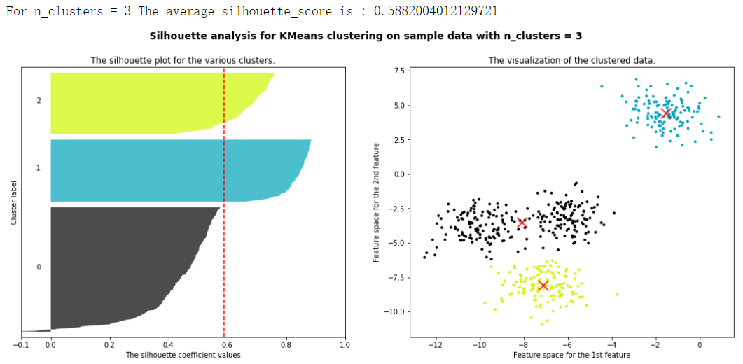
print("For n_clusters =", n_clusters,
      "The average silhouette_score is :", silhouette_avg)

sample_silhouette_values = silhouette_samples(X, cluster_labels)

y_lower = 10

for i in range(n_clusters):
    ith_cluster_silhouette_values = sample_silhouette_values[cluster_labels == i]
    ith_cluster_silhouette_values.sort()
    size_cluster_i = ith_cluster_silhouette_values.shape[0]
    y_upper = y_lower + size_cluster_i
    color = cm.nipy_spectral(float(i)/n_clusters)
    
    ax1.fill_betweenx(np.arange(y_lower, y_upper)
                      ,ith_cluster_silhouette_values
                      ,facecolor=color
                      ,alpha=0.7
                     )

    ax1.text(-0.05
             , y_lower + 0.5 * size_cluster_i
             , str(i))

    y_lower = y_upper + 10
    
ax1.set_title("The silhouette plot for the various clusters.")
ax1.set_xlabel("The silhouette coefficient values")
ax1.set_ylabel("Cluster label")

ax1.axvline(x=silhouette_avg, color="red", linestyle="--")

ax1.set_yticks([])

ax1.set_xticks([-0.1, 0, 0.2, 0.4, 0.6, 0.8, 1])

colors = cm.nipy_spectral(cluster_labels.astype(float) / n_clusters)

ax2.scatter(X[:, 0], X[:, 1]
            ,marker='o'
            ,s=8
            ,c=colors
           )

centers = clusterer.cluster_centers_
# Draw white circles at cluster centers
ax2.scatter(centers[:, 0], centers[:, 1], marker='x',
            c="red", alpha=1, s=200)

ax2.set_title("The visualization of the clustered data.")
ax2.set_xlabel("Feature space for the 1st feature")
ax2.set_ylabel("Feature space for the 2nd feature")

plt.suptitle(("Silhouette analysis for KMeans clustering on sample data"
              "with n_clusters = %d" % n_clusters),
             fontsize=14, fontweight='bold')
plt.show()

将上述过程包装成一个循环，可以得到：

from sklearn.cluster import KMeans
from sklearn.metrics import silhouette_samples, silhouette_score

import matplotlib.pyplot as plt
import matplotlib.cm as cm
import numpy as np

for n_clusters in [2,3,4,5,6,7]:
    n_clusters = n_clusters
    fig, (ax1, ax2) = plt.subplots(1, 2)
    fig.set_size_inches(18, 7)
    ax1.set_xlim([-0.1, 1])
    ax1.set_ylim([0, X.shape[0] + (n_clusters + 1) * 10])
    clusterer = KMeans(n_clusters=n_clusters, random_state=10).fit(X)
    cluster_labels = clusterer.labels_
    silhouette_avg = silhouette_score(X, cluster_labels)
    print("For n_clusters =", n_clusters,
          "The average silhouette_score is :", silhouette_avg)
    sample_silhouette_values = silhouette_samples(X, cluster_labels)
    y_lower = 10
    for i in range(n_clusters):
        ith_cluster_silhouette_values = sample_silhouette_values[cluster_labels == i]
        ith_cluster_silhouette_values.sort()
        size_cluster_i = ith_cluster_silhouette_values.shape[0]
        y_upper = y_lower + size_cluster_i
        color = cm.nipy_spectral(float(i)/n_clusters)
        ax1.fill_betweenx(np.arange(y_lower, y_upper)
                          ,ith_cluster_silhouette_values
                          ,facecolor=color
                          ,alpha=0.7
                         )
        ax1.text(-0.05
                 , y_lower + 0.5 * size_cluster_i
                 , str(i))
        y_lower = y_upper + 10

    ax1.set_title("The silhouette plot for the various clusters.")
    ax1.set_xlabel("The silhouette coefficient values")
    ax1.set_ylabel("Cluster label")
    ax1.axvline(x=silhouette_avg, color="red", linestyle="--")
    ax1.set_yticks([])
    ax1.set_xticks([-0.1, 0, 0.2, 0.4, 0.6, 0.8, 1])

    colors = cm.nipy_spectral(cluster_labels.astype(float) / n_clusters)
    ax2.scatter(X[:, 0], X[:, 1]
                ,marker='o'
                ,s=8
                ,c=colors
               )
    centers = clusterer.cluster_centers_
    # Draw white circles at cluster centers
    ax2.scatter(centers[:, 0], centers[:, 1], marker='x',
                c="red", alpha=1, s=200)
    
    ax2.set_title("The visualization of the clustered data.")
    ax2.set_xlabel("Feature space for the 1st feature")
    ax2.set_ylabel("Feature space for the 2nd feature")

    plt.suptitle(("Silhouette analysis for KMeans clustering on sample data "
                  "with n_clusters = %d" % n_clusters),
                 fontsize=14, fontweight='bold')
    plt.show()

3.2 重要参数 init & random_state & n_init ：初始质心怎么放好 ?

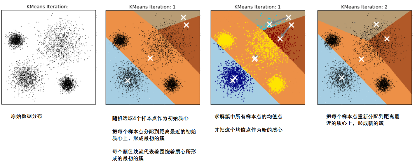
在 K-Means 中有一个重要的环节，就是放置初始质心。如果有足够的时间， K-means 一定会收敛，但 Inertia可能收敛到局部最小值。是否能够收敛到真正的最小值很大程度上取决于质心的初始化。 init就是用来帮助我们决定初始化方式的参数。

初始质心放置的位置不同，聚类的结果很可能也会不一样，一个好的质心选择可以让 K-Means避免更多的计算，让算法收敛稳定且更快。在之前讲解初始质心的放置时，我们是使用 ” 随机 “ 的方法在样本点中抽取 k个样本作为初始质心，这种方法显然不符合 ” 稳定且更快 “ 的需求。为此，我们可以使用 random_state参数来控制每次生成的初始质心都在相同位置，甚至可以画学习曲线来确定最优的 random_state 是哪个整数。

一个 random_state 对应一个质心随机初始化的随机数种子。如果不指定随机数种子，则 sklearn 中的K-means并不会只选择一个随机模式扔出结果，而会在每个随机数种子下运行多次，并使用结果最好的一个随机数种子来作为初始质心。我们可以使用参数 n_init 来选择，每个随机数种子下运行的次数。这个参数不常用到，默认 10次，如果我们希望运行的结果更加精确，那我们可以增加这个参数 n_init 的值来增加每个随机数种子下运行的次数。

然而这种方法依然是基于随机性的。

为了优化选择初始质心的方法， 2007 年 Arthur, David, and Sergei Vassilvitskii 三人发表了论文 “k-means++: The advantages of careful seeding” ，他们开发了 ”k-means ++“初始化方案，使得初始质心（通常）彼此远离，以此来引导出比随机初始化更可靠的结果。在 sklearn 中，我们使用参数 init ='k-means ++' 来选择使用 k-means ++作为质心初始化的方案。通常来说，我建议保留默认的 "k-means++" 的方法。

init ：可输入 "k-means++" ， "random" 或者一个 n 维数组。这是初始化质心的方法，默认 "k-means++" 。输入"k-means++" ：一种为 K 均值聚类选择初始聚类中心的聪明的办法，以加速收敛。如果输入了 n维数组，数组的形状应该是 (n_clusters ， n_features) 并给出初始质心。

random_state ：控制每次质心随机初始化的随机数种子

n_init ：整数，默认 10 ，使用不同的质心随机初始化的种子来运行 k-means 算法的次数。最终结果会是基于Inertia来计算的 n_init 次连续运行后的最佳输出

X.shape

y.shape

plus = KMeans(n_clusters = 10).fit(X)
plus.n_iter_  #12

random = KMeans(n_clusters = 10,init="random",random_state=420).fit(X)
random.n_iter_  #19

3.3 重要参数max_iter & tol：让迭代停下来

在之前描述 K-Means 的基本流程时我们提到过，当质心不再移动， Kmeans算法就会停下来。但在完全收敛之前，我们也可以使用 max_iter ，最大迭代次数，或者 tol ，两次迭代间 Inertia下降的量，这两个参数来让迭代提前停下来。有时候，当我们的 n_clusters选择不符合数据的自然分布，或者我们为了业务需求，必须要填入与数据的自然分布不合的 n_clusters ，提前让迭代停下来反而能够提升模型的表现。

max_iter ：整数，默认 300 ，单次运行的 k-means 算法的最大迭代次数

tol ：浮点数，默认 1e-4 ，两次迭代间 Inertia 下降的量，如果两次迭代之间 Inertia 下降的值小于 tol所设定的值，迭代就会停下

random = KMeans(n_clusters = 10,init="random",max_iter=10,random_state=420).fit(X)
y_pred_max10 = random.labels_
silhouette_score(X,y_pred_max10)
'''
0.3952586444034157
'''

random = KMeans(n_clusters = 10,init="random",max_iter=20,random_state=420).fit(X)
y_pred_max10 = random.labels_
silhouette_score(X,y_pred_max10)
'''
0.3401504537571701
'''

3.4 重要属性与重要接口

到这里，所有的重要参数就讲完了。在使用模型的过程中，我也向大家呈现了各种重要的属性与接口，在这一小节来复习一下：

3.5 函数cluster.k_means

sklearn.cluster.k_means ( X , n_clusters , sample_weight=None , init=’k-means++’ , precompute_distances=’auto’, n_init=10 , max_iter=300 , verbose=False , tol=0.0001 , random_state=None , copy_x=True , n_jobs=None,algorithm=’auto’ , return_n_iter=False )

函数 k_means 的用法其实和类非常相似，不过函数是输入一系列值，而直接返回结果。一次性地，函数 k_means会依次返回质心，每个样本对应的簇的标签， inertia 以及最佳迭代次数。

from sklearn.cluster import k_means
k_means(X,4,return_n_iter=True)

4 案例：聚类算法用于降维，KMeans的矢量量化应用

K-Means 聚类最重要的应用之一是非结构数据（图像，声音）上的矢量量化（VQ）。非结构化数据往往占用比较多的储存空间，文件本身也会比较大，运算非常缓慢，我们希望能够在保证数据质量的前提下，尽量地缩小非结构化数据的大小，或者简化非结构化数据的结构。矢量量化就可以帮助我们实现这个目的。KMeans聚类的矢量量化本质是一种降维运用，但它与我们之前学过的任何一种降维算法的思路都不相同。特征选择的降维是直接选取对模型贡献最大的特征， PCA 的降维是聚合信息，而 矢量量化的降维是在同等样本量上压缩信息的大小，即不改变特征的数目也不改变样本的数目，只改变在这些特征下的样本上的信息量。

对于图像来说，一张图片上的信息可以被聚类如下表示：

这是一组 40 个样本的数据，分别含有 40 组不同的信息 (x1,x2) 。我们将代表所有样本点聚成 4类，找出四个质心，我们认为，这些点和他们所属的质心非常相似，因此他们所承载的信息就约等于他们所在的簇的质心所承载的信息。

于是，我们可以使用每个样本所在的簇的质心来覆盖原有的样本，有点类似四舍五入的感觉，类似于用 1 来代替0.9和 0.8 。这样， 40 个样本带有的 40 种取值，就被我们压缩了 4 组取值，虽然样本量还是 40 个，但是这 40个样本所带的取值其实只有 4 个，就是分出来的四个簇的质心。

用 K-Means聚类中获得的质心来替代原有的数据，可以把数据上的信息量压缩到非常小，但又不损失太多信息。我们接下来就通过一张图图片的矢量量化来看一看 K-Means 如何实现压缩数据大小，却不损失太多信息量。

1. 导入需要的库

import numpy as np
import matplotlib.pyplot as plt
from sklearn.cluster import KMeans
from sklearn.metrics import pairwise_distances_argmin
    #对两个序列中的点进行距离匹配的函数
from sklearn.datasets import load_sample_image
    #导入图片数据所用的类
from sklearn.utils import shuffle #洗牌

2. 导入数据，探索数据


# 实例化，导入颐和园的图片
china = load_sample_image("china.jpg")

#查看数据类型 dtype('uint8')
china.dtype

china.shape
#长度 x 宽度 x 像素 > 三个数决定的颜色 (427, 640, 3)


#包含多少种不同的颜色?
newimage = china.reshape((427 * 640,3))

import pandas as pd
pd.DataFrame(newimage).drop_duplicates().shape

#我们现在有9W多种颜色 (96615, 3)

# 图像可视化
plt.figure(figsize=(15,15))
plt.imshow(china) #导入3维数组形成的图片

#查看模块中的另一张图片
flower = load_sample_image("flower.jpg")
plt.figure(figsize=(15,15))
plt.imshow(flower)

图像探索完毕，我们了解了，图像现在有 9W 多种颜色。我们希望来试试看，能否使用 K-Means 将颜色压缩到64种，还不严重损耗图像的质量。为此，我们要使用 K-Means 来将 9W 种颜色聚类成 64 类，然后使用 64个簇的质心来替代全部的 9W 种颜色，记得质心有着这样的性质：簇中的点都是离质心最近的样本点。

为了比较，我们还要画出随机压缩到 64 种颜色的矢量量化图像。我们需要随机选取64个样本点作为随机质心，计算原数据中每个样本到它们的距离来找出离每个样本最近的随机质心，然后用每个样本所对应的随机质心来替换原本的样本。两种状况下，我们观察图像可视化之后的状况，以查看图片信息的损失。

在这之前，我们需要把数据处理成 sklearn 中的 K-Means 类能够接受的数据。

3. 决定超参数，数据预处理

n_clusters = 64

china = np.array(china, dtype=np.float64) / china.max()
w, h, d = original_shape = tuple(china.shape)
assert d == 3
image_array = np.reshape(china, (w * h, d))

#plt.imshow在浮点数上表现非常优异，在这里我们把china中的数据，转换为浮点数，压缩到[0,1]之间
china = np.array(china, dtype=np.float64) / china.max()

#把china从图像格式，转换成矩阵格式
w, h, d = original_shape = tuple(china.shape)

#展示assert的功能
d_ = 3
assert d_ == 3, "一个格子中特征数不等于3"

image_array = np.reshape(china, (w * h, d)) #reshape是改变结构
image_array

image_array.shape

a = np.random.random((2,4))

a.reshape((4,2)) == np.reshape(a,(4,2))

np.reshape(a,(2,2,2)).shape

np.reshape(a,(8,1))

4. 对数据进行K-Means的矢量量化

image_array_sample = shuffle(image_array, random_state=0)[:1000]
kmeans = KMeans(n_clusters=n_clusters, random_state=0).fit(image_array_sample)
kmeans.cluster_centers_
labels = kmeans.predict(image_array)
labels.shape
image_kmeans = image_array.copy()
for i in range(w*h):
    image_kmeans[i] = kmeans.cluster_centers_[labels[i]]
image_kmeans
pd.DataFrame(image_kmeans).drop_duplicates().shape
image_kmeans = image_kmeans.reshape(w,h,d)
image_kmeans.shape

5. 对数据进行随机的矢量量化

centroid_random = shuffle(image_array, random_state=0)[:n_clusters]
labels_random = pairwise_distances_argmin(centroid_random,image_array,axis=0)
labels_random.shape
len(set(labels_random))
image_random = image_array.copy()
for i in range(w*h):
    image_random[i] = centroid_random[labels_random[i]]
image_random = image_random.reshape(w,h,d)
image_random.shape

6. 将原图，按 KMeans 矢量量化和随机矢量量化的图像绘制出来

plt.figure(figsize=(10,10))
plt.axis('off')
plt.title('Original image (96,615 colors)')
plt.imshow(china)
plt.figure(figsize=(10,10))
plt.axis('off')
plt.title('Quantized image (64 colors, K-Means)')
plt.imshow(image_kmeans)
plt.figure(figsize=(10,10))
plt.axis('off')
plt.title('Quantized image (64 colors, Random)')
plt.imshow(image_random)
plt.show()

本文内容由网友自发贡献，版权归原作者所有，本站不承担相应法律责任。如您发现有涉嫌抄袭侵权的内容，请联系:hwhale#tublm.com(使用前将#替换为@)