Ceres 自动求导解析-从原理到实践
文章目录
- Ceres 自动求导解析-从原理到实践
- 1.0 前言
- 2.0 Ceres求导简介
- 3.0 Ceres 自动求导原理
-
- 4.0 实践
- 4.1 Jet 的实现
- 4.2 多项式函数自动求导
- 4.3 BA 问题中的自动求导
- Reference
1.0 前言
Ceres 有一个自动求导功能,只要你按照Ceres要求的格式写好目标函数,Ceres会自动帮你计算精确的导数(或者雅克比矩阵),这极大节约了算法开发者的时间,但是笔者在使用的时候一直觉得这是个黑盒子,特别是之前在做深度学习的时候,神经网络本事是一个很盒模型了,再加上 pytorch 的自动求导,简直是黑上加黑。现在转入视觉SLAM方向,又碰到了 Ceres 的自动求导,是时候揭开其真实的面纱了。知其然并知其所以然才是一名算法工程师应有的基本素养。
2.0 Ceres求导简介
Ceres 一共有三种求导的方式提供给开发者,分别是:
-
解析求导,也就是手动计算出导数的解析形式。
例如有如下函数;
y
=
b
1
(
1
+
e
b
2
−
b
3
x
)
1
/
b
4
y = \frac{b_1}{(1+e^{b_2-b_3x})^{1/b_4}}
y=(1+eb2−b3x)1/b4b1
构建误差函数:
E
(
b
1
,
b
2
,
b
3
,
b
4
)
=
∑
i
f
2
(
b
1
,
b
2
,
b
3
,
b
4
;
x
i
,
y
i
)
=
∑
i
(
b
1
(
1
+
e
b
2
−
b
3
x
i
)
1
/
b
4
−
y
i
)
2
\begin{split}\begin{align} E(b_1, b_2, b_3, b_4) &= \sum_i f^2(b_1, b_2, b_3, b_4 ; x_i, y_i)\\ &= \sum_i \left(\frac{b_1}{(1+e^{b_2-b_3x_i})^{1/b_4}} - y_i\right)^2\\ \end{align}\end{split}
E(b1,b2,b3,b4)=i∑f2(b1,b2,b3,b4;xi,yi)=i∑((1+eb2−b3xi)1/b4b1−yi)2
对待优化变量的导数为:
D
1
f
(
b
1
,
b
2
,
b
3
,
b
4
;
x
,
y
)
=
1
(
1
+
e
b
2
−
b
3
x
)
1
/
b
4
D
2
f
(
b
1
,
b
2
,
b
3
,
b
4
;
x
,
y
)
=
−
b
1
e
b
2
−
b
3
x
b
4
(
1
+
e
b
2
−
b
3
x
)
1
/
b
4
+
1
D
3
f
(
b
1
,
b
2
,
b
3
,
b
4
;
x
,
y
)
=
b
1
x
e
b
2
−
b
3
x
b
4
(
1
+
e
b
2
−
b
3
x
)
1
/
b
4
+
1
D
4
f
(
b
1
,
b
2
,
b
3
,
b
4
;
x
,
y
)
=
b
1
log
(
1
+
e
b
2
−
b
3
x
)
b
4
2
(
1
+
e
b
2
−
b
3
x
)
1
/
b
4
\begin{split}\begin{align} D_1 f(b_1, b_2, b_3, b_4; x,y) &= \frac{1}{(1+e^{b_2-b_3x})^{1/b_4}}\\ D_2 f(b_1, b_2, b_3, b_4; x,y) &= \frac{-b_1e^{b_2-b_3x}}{b_4(1+e^{b_2-b_3x})^{1/b_4 + 1}} \\ D_3 f(b_1, b_2, b_3, b_4; x,y) &= \frac{b_1xe^{b_2-b_3x}}{b_4(1+e^{b_2-b_3x})^{1/b_4 + 1}} \\ D_4 f(b_1, b_2, b_3, b_4; x,y) & = \frac{b_1 \log\left(1+e^{b_2-b_3x}\right) }{b_4^2(1+e^{b_2-b_3x})^{1/b_4}} \end{align}\end{split}
D1f(b1,b2,b3,b4;x,y)D2f(b1,b2,b3,b4;x,y)D3f(b1,b2,b3,b4;x,y)D4f(b1,b2,b3,b4;x,y)=(1+eb2−b3x)1/b41=b4(1+eb2−b3x)1/b4+1−b1eb2−b3x=b4(1+eb2−b3x)1/b4+1b1xeb2−b3x=b42(1+eb2−b3x)1/b4b1log(1+eb2−b3x)
-
数值求导,当对变量增加一个微小的增量,然后观察此时的残差和原先残差的下降比例即可,其实就是导数的定义。
D
f
(
x
)
=
lim
h
→
0
f
(
x
+
h
)
−
f
(
x
)
h
Df(x) = \lim_{h \rightarrow 0} \frac{f(x + h) - f(x)}{h}
Df(x)=h→0limhf(x+h)−f(x)
当然其实也有两种形式对导数进行数值上的近似,第一种是Forward Differences:
D
f
(
x
)
≈
f
(
x
+
h
)
−
f
(
x
)
h
Df(x) \approx \frac{f(x + h) - f(x)}{h}
Df(x)≈hf(x+h)−f(x)
第二种是 Central Differences:
D
f
(
x
)
≈
f
(
x
+
h
)
−
f
(
x
−
h
)
2
h
Df(x) \approx \frac{f(x + h) - f(x - h)}{2h}
Df(x)≈2hf(x+h)−f(x−h)
Ceres 的官方文档上是认为第二种比第一种好的,但是其实官方还介绍了第三种,这里就不详说了,感兴趣的可以去看官方文档:Ridders’ Method。
这里有三种数值微分方法的效果对比,从右向左看:
[外链图片转存失败,源站可能有防盗链机制,建议将图片保存下来直接上传(img-thT2QEWp-1680337326032)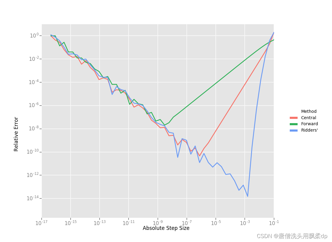
效果依次是
R
i
d
d
e
r
s
>
C
e
n
t
r
a
l
>
F
o
r
w
a
d
Ridders > Central > Forwad
Ridders>Central>Forwad
-
第三种则是今天要介绍的主角,自动求导。
3.0 Ceres 自动求导原理
3.1 官方解释
其实官方对自动求导做出了解释,但是笔者觉得写的不够直观,比较抽象,不过既然是官方出品,还是非常有必要去看一看的。http://ceres-solver.org/automatic_derivatives.html。
3.2 自我理解
\quad
这里笔者根据网上和官方的资料整理了一下自己的理解。Ceres 自动求导的核心是运算符的重载与Ceres自有的 Jet 变量。
举一个例子:
函数
f
(
x
)
=
h
(
x
)
∗
g
(
x
)
\mathrm{f}(\mathrm{x})=\mathrm{h}(\mathrm{x}) * \mathrm{~g}(\mathrm{x})
f(x)=h(x)∗ g(x) , 他的目标函数值为
h
(
x
)
∗
g
(
x
)
\mathrm{h}(\mathrm{x}) * \mathrm{~g}(\mathrm{x})
h(x)∗ g(x) , 导数为
f
′
(
x
)
=
h
′
(
x
)
g
(
x
)
+
h
(
x
)
g
′
(
x
)
\mathrm{f}^{\prime}(\mathrm{x})=\mathrm{h}^{\prime}(\mathrm{x}) \mathrm{g}(\mathrm{x})+\mathrm{h}(\mathrm{x}) \mathrm{g}^{\prime}(\mathrm{x})
f′(x)=h′(x)g(x)+h(x)g′(x)
其中
h
(
x
)
h(x)
h(x),
g
(
x
)
g(x)
g(x) 都是标量函数.
如果我们定义一种数据类型,
D
a
t
a
{
d
o
u
b
l
e
v
a
l
u
e
,
d
o
u
b
l
e
d
e
r
i
v
e
d
}
Data \{ double\ \ value, double\ \ derived \}
Data{double value,double derived}
并且对于数据类型 Data,重载乘法运算符
d
a
t
a
1
∗
d
a
t
a
2
=
[
d
a
t
a
1.
v
a
l
u
e
∗
d
a
t
a
2.
v
a
l
u
e
d
a
t
a
1.
d
e
r
i
v
e
d
∗
d
a
t
a
2.
v
a
l
u
e
+
d
a
t
a
1.
v
a
l
u
e
∗
d
a
t
a
2.
d
e
r
i
v
e
d
]
data1*data2=\begin{bmatrix} data1.value*data2.value \\ data1.derived*data2.value+data1.value*data2.derived \end{bmatrix}
data1∗data2=[data1.value∗data2.valuedata1.derived∗data2.value+data1.value∗data2.derived]
令
h
(
x
)
=
[
h
(
x
)
,
h
(
x
)
′
]
,
g
(
x
)
=
[
g
(
x
)
,
g
(
x
)
′
]
h(x) =[h(x),{h(x)}' ] , g(x)=[g(x),{g(x)' }]
h(x)=[h(x),h(x)′],g(x)=[g(x),g(x)′]。
f
(
x
)
=
h
(
x
)
∗
g
(
x
)
f(x)=h(x) * g(x)
f(x)=h(x)∗g(x), 那么f_x.derived 就是
f
(
x
)
f(x)
f(x)的导数,f_x.value 即为
f
(
x
)
f(x)
f(x)的数值。value 储存变量的函数值, derived 储存变量对
x
\mathrm{x}
x 的导数。类似,如果我们对数据类型 Data 重载所有可能用到的运算符. “
+
−
∗
/
log
,
exp
,
⋯
+- * / \log , \exp , \cdots
+−∗/log,exp,⋯” 。那么在变量
h
(
x
)
,
g
(
x
)
h(x),g(x)
h(x),g(x)经过任意次运算后,
r
e
s
u
l
t
=
h
(
x
)
+
g
(
x
)
∗
h
(
x
)
+
e
x
p
(
h
(
x
)
)
…
result=h(x)+g(x)*h(x)+exp(h(x))…
result=h(x)+g(x)∗h(x)+exp(h(x))…, 任然能获得函数值 result.value 和他的导数值 result.derived,这就是Ceres 自动求导的原理。
上面讲的都是单一自变量的自动求导,对于多元函数
f
(
x
i
)
f(x_i)
f(xi)。对于n 元函数,Data 里面的 double derived 就替换为 double* derived,derived[i] 为对于第i个自变量的导数值。
并且对于数据类型 Data,乘法运算符重载为
d
a
t
a
1
∗
d
a
t
a
2
=
[
d
a
t
a
1.
v
a
l
u
e
∗
d
a
t
a
2.
v
a
l
u
e
d
e
r
i
v
e
d
[
i
]
=
d
a
t
a
1.
d
e
r
i
v
e
d
[
i
]
∗
d
a
t
a
2.
v
a
l
u
e
+
d
a
t
a
1.
v
a
l
u
e
∗
d
a
t
a
2.
d
e
r
i
v
e
d
[
i
]
]
data1*data2=\begin{bmatrix} data1.value*data2.value \\ derived[i]=data1.derived[i]*data2.value+data1.value*data2.derived[i] \end{bmatrix}
data1∗data2=[data1.value∗data2.valuederived[i]=data1.derived[i]∗data2.value+data1.value∗data2.derived[i]]
其余的运算符重载方法也做相应改变。这样对多元函数的自动求导问题也就解决了。Ceres 里面的Jet 数据类型类似于 这里Data 类型,并且Ceres 对Jet 数据类型进行了几乎所有数学运算符的重载,以达到自动求导的目的。
4.0 实践
4.1 Jet 的实现
这里我们模仿 Ceres 实现了 Jet ,并准备了两个具体的示例程序,Jet 具体代码在 ceres_jet.hpp 中,包装成了一个头文件,在使用的时候进行调用即可。这里也包含了一个 ceres_rotation.hpp 的头文件,是为了我们的第二个例子实现。具体代码如下:
#ifndef _CERES_JET_HPP__
#define _CERES_JET_HPP__
#include <math.h>
#include <stdio.h>

#include <eigen3/Eigen/Core>
#include <eigen3/Eigen/Dense>
#include <eigen3/Eigen/Sparse>
#include "eigen3/Eigen/Eigen"
#include "eigen3/Eigen/SparseQR"
#include <fstream>
#include <iostream>
#include <map>
#include <queue>
#include <set>
#include <vector>
#include "ceres_rotation.hpp"

#include "algorithm"
#include "stdlib.h"

template <int N>
struct jet
{
  Eigen::Matrix<double, N, 1> v;
  double a;
  jet() : a(0.0) {}
  jet(const double& value) : a(value) { v.setZero(); }
  EIGEN_STRONG_INLINE jet(const double& value,
                          const Eigen::Matrix<double, N, 1>& v_)
      : a(value), v(v_)
  {
  }
  jet(const double value, const int index)
  {
    v.setZero();
    a = value;
    v(index, 0) = 1.0;
  }
  void init(const double value, const int index)
  {
    v.setZero();
    a = value;
    v(index, 0) = 1.0;
  }
};
/****************jet overload******************/
// for the camera BA,the autodiff only need overload the operator :jet+jet
// number+jet -jet jet-number jet*jet number/jet jet/jet sqrt(jet) cos(jet)
// sin(jet)  +=(jet) overload jet + jet
template <int N>
inline jet<N> operator+(const jet<N>& A, const jet<N>& B)
{
  return jet<N>(A.a + B.a, A.v + B.v);
}  // end jet+jet

// overload number + jet
template <int N>
inline jet<N> operator+(double A, const jet<N>& B)
{
  return jet<N>(A + B.a, B.v);
}  // end number+jet

template <int N>
inline jet<N> operator+(const jet<N>& B, double A)
{
  return jet<N>(A + B.a, B.v);
}  // end number+jet

// overload jet-number
template <int N>
inline jet<N> operator-(const jet<N>& A, double B)
{
  return jet<N>(A.a - B, A.v);
}
// overload number * jet because jet *jet need A.a *B.v+B.a*A.v.So the number
// *jet is required
template <int N>
inline jet<N> operator*(double A, const jet<N>& B)
{
  return jet<N>(A * B.a, A * B.v);
}
template <int N>
inline jet<N> operator*(const jet<N>& A, double B)
{
  return jet<N>(B * A.a, B * A.v);
}
// overload -jet
template <int N>
inline jet<N> operator-(const jet<N>& A)
{
  return jet<N>(-A.a, -A.v);
}
template <int N>
inline jet<N> operator-(double A, const jet<N>& B)
{
  return jet<N>(A - B.a, -B.v);
}
template <int N>
inline jet<N> operator-(const jet<N>& A, const jet<N>& B)
{
  return jet<N>(A.a - B.a, A.v - B.v);
}
// overload jet*jet
template <int N>
inline jet<N> operator*(const jet<N>& A, const jet<N>& B)
{
  return jet<N>(A.a * B.a, B.a * A.v + A.a * B.v);
}
// overload number/jet
template <int N>
inline jet<N> operator/(double A, const jet<N>& B)
{
  return jet<N>(A / B.a, -A * B.v / (B.a * B.a));
}
// overload jet/jet
template <int N>
inline jet<N> operator/(const jet<N>& A, const jet<N>& B)
{
  // This uses:
  //
  //   a + u   (a + u)(b - v)   (a + u)(b - v)
  //   ----- = -------------- = --------------
  //   b + v   (b + v)(b - v)        b^2
  //
  // which holds because v*v = 0.
  const double a_inverse = 1.0 / B.a;
  const double abyb = A.a * a_inverse;
  return jet<N>(abyb, (A.v - abyb * B.v) * a_inverse);
}
// sqrt(jet)
template <int N>
inline jet<N> sqrt(const jet<N>& A)
{
  double t = std::sqrt(A.a);

  return jet<N>(t, 1.0 / (2.0 * t) * A.v);
}
// cos(jet)
template <int N>
inline jet<N> cos(const jet<N>& A)
{
  return jet<N>(std::cos(A.a), -std::sin(A.a) * A.v);
}
template <int N>
inline jet<N> sin(const jet<N>& A)
{
  return jet<N>(std::sin(A.a), std::cos(A.a) * A.v);
}
template <int N>
inline bool operator>(const jet<N>& f, const jet<N>& g)
{
  return f.a > g.a;
}

#endif //_CERES_JET_HPP__
#ifndef CERES_ROTATION_HPP_
#define CERES_ROTATION_HPP_
#include <iostream>

template <typename T>
inline T DotProduct(const T x[3], const T y[3])
{
  return (x[0] * y[0] + x[1] * y[1] + x[2] * y[2]);
}

template <typename T>
inline void AngleAxisRotatePoint(const T angle_axis[3], const T pt[3],
                                 T result[3])
{
  const T theta2 = DotProduct(angle_axis, angle_axis);
  if (theta2 > T(std::numeric_limits<double>::epsilon()))
  {
    // Away from zero, use the rodriguez formula
    //
    //   result = pt costheta +
    //            (w x pt) * sintheta +
    //            w (w . pt) (1 - costheta)
    //
    // We want to be careful to only evaluate the square root if the
    // norm of the angle_axis vector is greater than zero. Otherwise
    // we get a division by zero.
    //
    const T theta = sqrt(theta2);
    const T costheta = cos(theta);
    const T sintheta = sin(theta);
    const T theta_inverse = T(1.0) / theta;

    const T w[3] = {angle_axis[0] * theta_inverse,
                    angle_axis[1] * theta_inverse,
                    angle_axis[2] * theta_inverse};

    // Explicitly inlined evaluation of the cross product for
    // performance reasons.
    const T w_cross_pt[3] = {w[1] * pt[2] - w[2] * pt[1],
                             w[2] * pt[0] - w[0] * pt[2],
                             w[0] * pt[1] - w[1] * pt[0]};
    const T tmp =
        (w[0] * pt[0] + w[1] * pt[1] + w[2] * pt[2]) * (T(1.0) - costheta);

    result[0] = pt[0] * costheta + w_cross_pt[0] * sintheta + w[0] * tmp;
    result[1] = pt[1] * costheta + w_cross_pt[1] * sintheta + w[1] * tmp;
    result[2] = pt[2] * costheta + w_cross_pt[2] * sintheta + w[2] * tmp;
  }
  else
  {
    // Near zero, the first order Taylor approximation of the rotation
    // matrix R corresponding to a vector w and angle w is
    //
    //   R = I + hat(w) * sin(theta)
    //
    // But sintheta ~ theta and theta * w = angle_axis, which gives us
    //
    //  R = I + hat(w)
    //
    // and actually performing multiplication with the point pt, gives us
    // R * pt = pt + w x pt.
    //
    // Switching to the Taylor expansion near zero provides meaningful
    // derivatives when evaluated using Jets.
    //
    // Explicitly inlined evaluation of the cross product for
    // performance reasons.
    const T w_cross_pt[3] = {angle_axis[1] * pt[2] - angle_axis[2] * pt[1],
                             angle_axis[2] * pt[0] - angle_axis[0] * pt[2],
                             angle_axis[0] * pt[1] - angle_axis[1] * pt[0]};

    result[0] = pt[0] + w_cross_pt[0];
    result[1] = pt[1] + w_cross_pt[1];
    result[2] = pt[2] + w_cross_pt[2];
  }
}

#endif  // CERES_ROTATION_HPP_
4.2 多项式函数自动求导
这里我们准备了两个实践案例,一个是对下面的函数进行自动求导,求在
f
(
1
,
2
)
f(1,2)
f(1,2) 处的导数。
f
(
x
,
y
)
=
2
x
2
+
3
y
3
+
3
f(x,y)=2x^2+3y^3+3
f(x,y)=2x2+3y3+3
代码如下:
#include <eigen3/Eigen/Core>
#include <eigen3/Eigen/Dense>

#include "ceres_jet.hpp"

int main(int argc, char const *argv[])
{
  /// f(x,y) = 2*x^2 + 3*y^3 + 3
  /// 残差的维度,变量1的维度,变量2的维度
  const int N = 1, N1 = 1, N2 = 1;
  Eigen::Matrix<double, N, N1> jacobian_parameter1;
  Eigen::Matrix<double, N, N2> jacobian_parameter2;
  Eigen::Matrix<double, N, 1> jacobi_residual;

  /// 模板参数为向量的维度,一定要是 N1+N2
  /// 也就是总的变量的维度,因为要存储结果(残差)
  /// 对于每个变量的导数值
  /// 至于为什么有 N1 个 jet 表示 var_x
  /// 假设变量 1 的维度为 N1,则残差对该变量的导数的维度是一个 N*N1 的矩阵
  /// 一个 jet<N1 + N2> 只能表示变量中的某一个在当前点的导数和值
  jet<N1 + N2> var_x[N1];
  jet<N1 + N2> var_y[N2];
	jet<N1 + N2> residual[N];
	/// 假设我们求上面的方程在 (x,y)->(1.0,2.0) 处的导数值
	double var_x_init_value[N1] = {1.0};
	double var_y_init_value[N1] = {2.0};

  for (int i = 0; i < N1; i++)
  {
    var_x[i].init(var_x_init_value[i], i);
  }
  for (int i = 0; i < N2; i++)
  {
    var_y[i].init(var_y_init_value[i], i + N1);
  }
	/// f(x,y) = 2*x^2 + 3*y^3 + 3
	/// f_x` = 4x
	/// f_y` = 9 * y^2
	residual[0] = 2.0 * var_x[0] * var_x[0]  + 3.0 * var_y[0] * var_y[0] * var_y[0] + 3.0;
	std::cout << "residual: " << residual[0].a << std::endl;
	std::cout << "jacobian: " << residual[0].v.transpose() << std::endl;
	/// residual: 29
	/// jacobian:  4 36
  return 0;
}
4.3 BA 问题中的自动求导
这里是用的 Bal 数据集中的某个观测构建的误差项求导
#include "ceres_jet.hpp"

class costfunction
{
 public:
  double x_;
  double y_;
  costfunction(double x, double y) : x_(x), y_(y) {}
  template <class T>
  void Evaluate(const T* camera, const T* point, T* residual)
  {
    T result[3];
    AngleAxisRotatePoint(camera, point, result);
    result[0] = result[0] + camera[3];
    result[1] = result[1] + camera[4];
    result[2] = result[2] + camera[5];
    T xp = -result[0] / result[2];
    T yp = -result[1] / result[2];
    T r2 = xp * xp + yp * yp;
    T distortion = 1.0 + r2 * (camera[7] + camera[8] * r2);
    T predicted_x = camera[6] * distortion * xp;
    T predicted_y = camera[6] * distortion * yp;
    residual[0] = predicted_x - x_;
    residual[1] = predicted_y - y_;
  }
};

int main(int argc, char const* argv[])
{
  const int N = 2, N1 = 9, N2 = 3;
  Eigen::Matrix<double, N, N1> jacobi_parameter_1;
  Eigen::Matrix<double, N, N2> jacobi_parameter_2;
  Eigen::Matrix<double, N, 1> jacobi_residual;
  costfunction* costfunction_ = new costfunction(-3.326500e+02, 2.620900e+02);
  jet<N1 + N2> cameraJet[N1];
  jet<N1 + N2> pointJet[N2];
  double params_1[N1] = {
      1.5741515942940262e-02,  -1.2790936163850642e-02, -4.4008498081980789e-03,
      -3.4093839577186584e-02, -1.0751387104921525e-01, 1.1202240291236032e+00,
      3.9975152639358436e+02,  -3.1770643852803579e-07, 5.8820490534594022e-13};
  double params_2[N2] = {-0.612000157172, 0.571759047760, -1.847081276455};
  for (int i = 0; i < N1; i++)
  {
    cameraJet[i].init(params_1[i], i);
  }
  for (int i = 0; i < N2; i++)
  {
    pointJet[i].init(params_2[i], i + N1);
  }
  jet<N1 + N2>* residual = new jet<N1 + N2>[N];
  costfunction_->Evaluate(cameraJet, pointJet, residual);
  for (int i = 0; i < N; i++)
  {
    jacobi_residual(i, 0) = residual[i].a;
  }
  for (int i = 0; i < N; i++)
  {
    jacobi_parameter_1.row(i) = residual[i].v.head(N1);
    jacobi_parameter_2.row(i) = residual[i].v.tail(N2);
  }
  /*
  real result:
  jacobi_parameter_1:
   -283.512    -1296.34    -320.603     551.177 0.000204691    -471.095   -0.854706    -409.362    -490.465
    1242.05      220.93    -332.566 0.000204691     551.177       376.9     0.68381     327.511     392.397
  jacobi_parameter_2:
  545.118 -5.05828 -478.067
  2.32675  557.047  368.163
  jacobi_residual:
  -9.02023
    11.264
   */
  std::cout << "jacobi_parameter_1: \n" << jacobi_parameter_1 << std::endl;
  std::cout << "jacobi_parameter_2: \n" << jacobi_parameter_2 << std::endl;
  std::cout << "jacobi_residual: \n" << jacobi_residual << std::endl;
  delete (residual);
  return 0;
}
Reference
- http://ceres-solver.org/
- https://blog.csdn.net/u012260559/article/details/105878468
- https://www.ngui.cc/article/show-902862.html?action=onClick
本文内容由网友自发贡献,版权归原作者所有,本站不承担相应法律责任。如您发现有涉嫌抄袭侵权的内容,请联系:hwhale#tublm.com(使用前将#替换为@)