时序分析 30 金融资产预测 - 蒙特卡洛模拟

2023-10-26

金融资产预测

蒙特卡洛模拟

商业经营活动中经常需要预测其收入、成本和利润。企业中的金融团队很可能会被要求构建金融模型进行场景分析，例如在不同的假设的情况下分析最好的情况、正常情况和最差的情况。这样做的目的主要是为管理层提供在不同的市场情况下公司的业务的营收情况的预览。但是构建类似模型的一个显著问题就是我们通常难以估算各种场景出现的概率。本文中，我们探讨使用Python语言应用蒙特卡洛模拟来缓解前面所说的问题，并且提供公司到达其目标的似然估计。

蒙特卡洛模拟简介

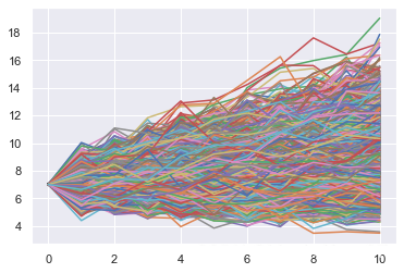
    蒙特卡洛模拟通常被用来对不同结果的概率建模，这些结果因为一些相关的随机因素而难以预测。蒙特卡洛模拟的构建方法千差万别，但它们一般会根据一个假设的概率分布来生成随机的输入，然后根据这些输入来计算或者聚合出结果。简单来说，蒙特卡洛模拟就是至少运行模型上千次，得到一系列的结果，这些结果会呈现一个概率分布，后结合所有结果来组成一个概况。
    蒙特卡洛模拟的应用非常广，尤其是在金融领域，例如期权定价模型(Black Scholes Model)、违约风险分析（在线价值，Value at Risk)等。
    蒙特卡洛模拟的简单模型应是单根或者随机步行模型。随机步行模型通过变量历史值加上一个随机噪声来得到当前的结果，该随机噪声通常被定义为是一个标准正态分布。请见下式：
S t = S t − 1 + Z t , S 0 = 0 , Z t ∼ N ( 0 , 1 ) S_t=S_{t-1}+Z_t,S_0=0,Z_t \sim N(0,1) St=St−1+Zt,S0=0,Zt∼N(0,1)

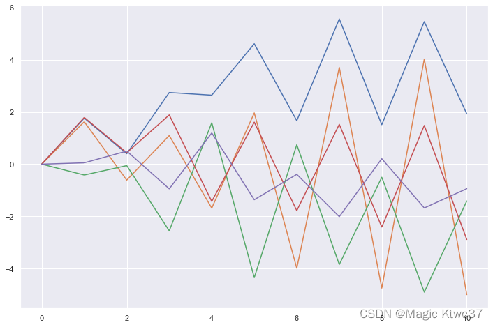
随机步行

import numpy as np
import matplotlib.pyplot as plt
import seaborn as sns
%matplotlib inline
sns.set()

monte_carlo = []
for i in range(5):
    forecasts = [0]
    np.random.seed(i)
    for j in range(10):
        forecast = forecasts[j-1] + np.random.normal()
        forecasts.append(forecast)
    monte_carlo.append(forecasts)
plt.figure(figsize=(12,8))
plt.plot(np.array(monte_carlo).T);

在这里插入图片描述
上图展示了10个模拟结果。

几何布朗运动

蒙特卡洛模拟中常用的复杂模型当属几何布朗运动(Geometric Brownian Motion,GBM)。GBM模型假设未来与历史是无关的，如果将这个模型应用于金融资产价格分析场景中，它假设过去的价值信息已经融入到了现在的价格中，而且当前的价格变动条件无关于过去的任何价格变动。

GBM模型公式如下：
S t = S 0 e x p ( ( μ − σ 2 / 2 ) t − σ × W t ) S_t=S_0exp((\mu-\sigma^2/2)t-\sigma\times W_t) St=S0exp((μ−σ2/2)t−σ×Wt)
W t − W t − 1 = d t Z t W_t-W_{t-1}=\sqrt{dt}Z_t Wt−Wt−1=dt Zt
Z t ∼ N ( 0 , 1 ) Z_t\sim N(0,1) Zt∼N(0,1)

这里， μ \mu μ为偏移率，确定了随机过程平均值的变化， σ \sigma σ是该变化的波动。
GBM模型亦可以写成如下形式：
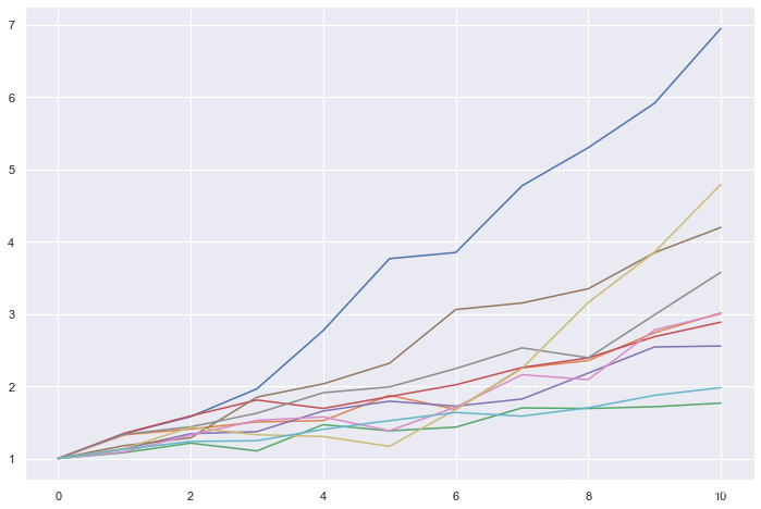
S t = s t − 1 e x p ( ( μ − σ 2 / 2 ) d t − σ d t Z t ) S_t=s_{t-1}exp((\mu-\sigma^2/2)dt-\sigma \sqrt{dt}Z_t) St=st−1exp((μ−σ2/2)dt−σdt Zt)
下图展示了GBM模型的10个模拟，参数为：
S 0 = 1 , μ = 0.05 , σ = 0.2 S_0=1,\mu=0.05,\sigma=0.2 S0=1,μ=0.05,σ=0.2

monte_carlo = []
no_of_iter = 10
sigma = 0.2
mu = 0.5
delta_t = 0.25
for i in range(no_of_iter):
    np.random.seed(i)
    forecasts = [1]
    for j in range(10):
        forecast = forecasts[j]*np.exp((mu-sigma**2/2)*(delta_t) + sigma*np.sqrt(delta_t)*np.random.normal())
        forecasts.append(forecast)
    monte_carlo.append(forecasts)
x = np.array(monte_carlo)
plt.figure(figsize=(12,8))
plt.plot(x.T);

在这里插入图片描述

金融预测应用蒙特卡洛模拟

我们先建立一个简单的金融模型，
P r o f i t = R e v e n u e − F i x e d C o s t − V a r i a b l e C o s t Profit=Revenue-FixedCost-VariableCost Profit=Revenue−FixedCost−VariableCost

我们假设在Year 0,收入为 10，固定成本为 2，可变成本为收入的10%。我们又假设收入在未来的10年每年会增长2%，得到一个利润增长的确定的路径，如下图：

revenues = []
gross_profits = []
mu = 0.02
revenue = [10]
fixed_cost = [2]
var_cost = [1]
for j in range(10):
    revenue.append(revenue[j]*(1+mu))
    fixed_cost.append(fixed_cost[j])
    var_cost.append(revenue[j]*0.1)
    gross_profit = [x - y - z for x, y, z in zip(revenue, fixed_cost, var_cost)]
plt.figure(figsize=(12,8))
plt.plot(np.array(gross_profit));

在这里插入图片描述
现在我们引入蒙特卡洛模拟，假设收入符合GBM模型，增长率为2%，波动率为5%，模拟10000次。

no_of_iter = 10000
delta_t = 1
revenues = []
gross_profits = []
for i in range(no_of_iter):
    revenue = [10]
    mu = 0.02
    sigma = 0.05
    fixed_cost = [2]
    var_cost = [1]
    np.random.seed(i)
    for j in range(10):
        revenue.append(revenue[j]*np.exp((mu-sigma**2/2)*(delta_t) + sigma*np.sqrt(delta_t)*np.random.normal()))
        fixed_cost.append(fixed_cost[j])
        var_cost.append(revenue[j]*0.1)
        gross_profit = [x - y - z for x, y, z in zip(revenue, fixed_cost, var_cost)]
    revenues.append(revenue)
    gross_profits.append(gross_profit)
gross_profits = np.array(gross_profits)
gross_profits.mean(axis=0)
plt.figure(figsize=(16,12))
plt.plot(np.array(gross_profits).T);

在这里插入图片描述
我们已经有了10000个结果，可以总结这些结果，得到利润的95%的区间，以下图阴影面积表示。

def interval_chart(gross_profits):
    fig, ax = plt.subplots(figsize=(12,8))
    x = np.arange(11)
    y1 = np.percentile(gross_profits, 97.5, axis=0)
    y2 = np.percentile(gross_profits, 2.5, axis=0)
    ax.plot(y1, color = '#1063B6')
    ax.plot(y2, color = '#4D99ED')
    ax.fill_between(x, y1, y2, alpha=0.4)
    ax.legend(labels=["97.5%","2.5%"])
    return plt.show()

interval_chart(gross_profits)

在这里插入图片描述
在金融预测中应用蒙特卡洛模拟，我们可以更好地估算未来利润在某个特定区间之内的概率，当然是以我们对增长率和波动的假设为前提的。对于增长率和波动率，我们可以通过历史数据进行估算或者例如类似的行业比较等其他相关金融变量，后可根据预期做一定调整。

我们可以进一步丰富这个模型。例如，我们假设可变成本服从一个均值为10%，标准差为5%的标准正态分布。从下图可以看出，增加了参数的复杂性使模型的结果更加波动。

no_of_iter = 10000
delta = 1
revenues = []
gross_profits = []
for i in range(no_of_iter):
    revenue = [10]
    mu = 0.02
    sigma = 0.05
    fixed_cost = [2]
    var_cost = [1]
    np.random.seed(i)
    for j in range(10):
        revenue.append(revenue[j]*np.exp((mu-sigma**2/2)*(delta_t) + sigma*np.sqrt(delta_t)*np.random.normal()))
        fixed_cost.append(fixed_cost[j])
        var_cost.append(revenue[j]*np.random.normal(0.1,0.05))
        gross_profit = [x - y - z for x, y, z in zip(revenue, fixed_cost, var_cost)]
    revenues.append(revenue)
    gross_profits.append(gross_profit)
gross_profits = np.array(gross_profits)
gross_profits.mean(axis=0)
plt.plot(np.array(gross_profits).T)

interval_chart(gross_profits)

在这里插入图片描述

当金融模型越来越复杂时，模型的各种输入变量都可以以随机变量的方法建模。例如，我们如果预测交通运输业的利润时，可以把油价作为一个可变成本的主要成分；也可考虑把原油的远期大宗商品价格的变化考虑进GBM模型中。

本文内容由网友自发贡献，版权归原作者所有，本站不承担相应法律责任。如您发现有涉嫌抄袭侵权的内容，请联系:hwhale#tublm.com(使用前将#替换为@)