使用IMU和llidar或者相机进行多传感器融合的slam方案中,主要分为紧耦合和松耦合方案。目前,主流的方案都是紧耦合的。而紧耦合方案中主要分为基于滤波(比如,ESKF)和基于优化的方案。
简介
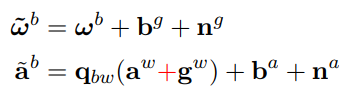
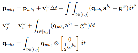
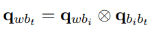
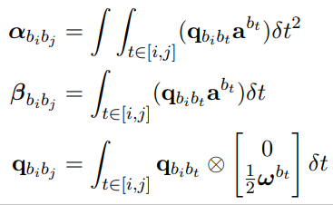
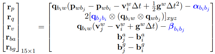
IMU的使用一般是对其测得的加速度,角速度进行积分,从而推算出机器人的位姿。但是,由于积分关系,IMU的积分所得的位姿飘移会随着积分时间的增大而增大。另一方面,当优化方法优化了历史时刻的位姿之后,之后时刻的IMU积分值需要重新进行积分,计算量大。因此,IMU预积分就被提出,以解决以上问题。IMU预积分简单来说就是描述了lidar帧(或者相机帧)之间(时间间隔比较短,比如lidar帧间间隔通常为100ms),IMU数据的观测量。其只跟上一帧时刻的IMU状态量相关,因此,在进行优化过程中,计算量较小。作为观测量,IMU预积分自然是作为一个约束用于slam位姿优化。
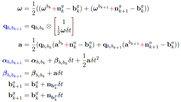
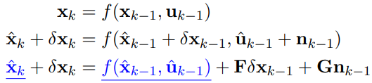
公式推导
IMU模型:
w
b
w^b
w b
a
w
a^w
a w
b
g
b^g
b g
b
a
b^a
b a
n
g
n^g
n g
n
a
n^a
n a
a
~
b
\widetilde{a}^b
a
b
w
~
b
\widetilde{w}^b
w
b
f
(
x
k
−
1
,
u
k
−
1
)
f(x_{k-1},u_{k-1})
f ( x k − 1 , u k − 1 )
x
^
k
−
1
\hat{x}_{k-1}
x ^ k − 1
简介
gtsam是通过因子图这个模型实现优化的。因此,在使用gtsam解决一个优化问题时,就需要构建相应的因子图。
IMU预积分类
gtsam中的一种IMU预积分实现类是PreintegratedImuMeasurements。其中,
void PreintegrationBase :: integrateMeasurement ( const Vector3& measuredAcc,
const Vector3& measuredOmega, double dt) {
Matrix9 A;
Matrix93 B, C;
update ( measuredAcc, measuredOmega, dt, & A, & B, & C) ;
}
这个成员函数,接受IMU的加速度,角速度测量值以及imu测量值之间的时间间隔。然后,计算相应的预积分量和噪声传播的雅克比矩阵。
NavState PreintegrationBase :: predict ( const NavState& state_i,
const imuBias:: ConstantBias& bias_i, OptionalJacobian< 9 , 9 > H1,
OptionalJacobian< 9 , 6 > H2) const {
Matrix96 D_biasCorrected_bias;
Vector9 biasCorrected = biasCorrectedDelta ( bias_i,
H2 ? & D_biasCorrected_bias : nullptr ) ;
Matrix9 D_delta_state, D_delta_biasCorrected;
Vector9 xi = state_i. correctPIM ( biasCorrected, deltaTij_, p ( ) . n_gravity,
p ( ) . omegaCoriolis, p ( ) . use2ndOrderCoriolis, H1 ? & D_delta_state : nullptr ,
H2 ? & D_delta_biasCorrected : nullptr ) ;
Matrix9 D_predict_state, D_predict_delta;
NavState state_j = state_i. retract ( xi,
H1 ? & D_predict_state : nullptr ,
H2 || H2 ? & D_predict_delta : nullptr ) ;
if ( H1)
* H1 = D_predict_state + D_predict_delta * D_delta_state;
if ( H2)
* H2 = D_predict_delta * D_delta_biasCorrected * D_biasCorrected_bias;
return state_j;
}
这个成员函数根据预积分量以及输入的PVQ,Bias进行当前时刻imu积分值计算。计算得到的结果可以作为相应节点的初始值。
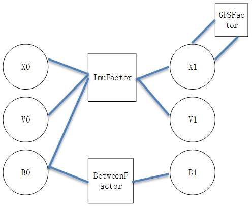
gtsam因子图构建
NonlinearFactorGraph* graph = new NonlinearFactorGraph ( ) ;
graph-> addPrior ( X ( correction_count) , prior_pose, pose_noise_model) ;
graph-> addPrior ( V ( correction_count) , prior_velocity, velocity_noise_model) ;
graph-> addPrior ( B ( correction_count) , prior_imu_bias, bias_noise_model) ;
先实例化因子图对象,而后加入先验节点。
std:: shared_ptr< PreintegrationType> preintegrated =
std:: make_shared < PreintegratedImuMeasurements> ( p, prior_imu_bias) ;
创建imu预积分对象。
preintegrated-> integrateMeasurement ( imu. head < 3 > ( ) , imu. tail < 3 > ( ) , dt) ;
根据imu观测值的输入,进行imu预积分计算。直到获得位姿观测值。
auto preint_imu =
dynamic_cast < const PreintegratedImuMeasurements& > ( * preintegrated) ;
ImuFactor imu_factor ( X ( correction_count - 1 ) , V ( correction_count - 1 ) ,
X ( correction_count) , V ( correction_count) ,
B ( correction_count - 1 ) , preint_imu) ;
graph-> add ( imu_factor) ;
imuBias:: ConstantBias zero_bias ( Vector3 ( 0 , 0 , 0 ) , Vector3 ( 0 , 0 , 0 ) ) ;
graph-> add ( BetweenFactor < imuBias:: ConstantBias> (
B ( correction_count - 1 ) , B ( correction_count) , zero_bias,
bias_noise_model) ) ;
当获得位姿观测值(比如,GPS数据,lidar匹配的位姿等)时,就利用imu预积分对象构建imu因子。
auto correction_noise = noiseModel:: Isotropic :: Sigma ( 3 , 1.0 ) ;
GPSFactor gps_factor ( X ( correction_count) ,
Point3 ( gps ( 0 ) ,
gps ( 1 ) ,
gps ( 2 ) ) ,
correction_noise) ;
graph-> add ( gps_factor) ;
同时,利用位姿观测值构建相应的因子。
LevenbergMarquardtOptimizer optimizer ( * graph, initial_values) ;
result = optimizer. optimize ( ) ;
gtsam中NonlinearConjugateGradientOptimizer这个优化器的optimize()源码如下所示:
const Values& NonlinearConjugateGradientOptimizer :: optimize ( ) {
System system ( graph_) ;
Values newValues;
int iterations;
boost:: tie ( newValues, iterations) =
nonlinearConjugateGradient ( system, state_-> values, params_, false ) ;
state_. reset ( new State ( std:: move ( newValues) , graph_. error ( newValues) , iterations) ) ;
return state_-> values;
}
其中,nonlinearConjugateGradient函数就是调用因子图中的因子类对象,计算残差和相应的雅可比矩阵。然后,使用该优化器的优化算法进行节点变量优化。具体说明雅可比矩阵的实现过程。
static VectorValues gradientInPlace ( const NonlinearFactorGraph & nfg,
const Values & values) {
GaussianFactorGraph:: shared_ptr linear = nfg. linearize ( values) ;
return linear-> gradientAtZero ( ) ;
}
其中,主要是因子图对象调用linearize()函数。linearize()函数部分源码如下所示:
GaussianFactorGraph:: shared_ptr NonlinearFactorGraph :: linearize ( const Values& linearizationPoint) const
{
gttic ( NonlinearFactorGraph_linearize) ;
GaussianFactorGraph:: shared_ptr linearFG = boost:: make_shared < GaussianFactorGraph> ( ) ;
# ifdef GTSAM_USE_TBB -> resize ( size ( ) ) ;
TbbOpenMPMixedScope threadLimiter;
tbb:: parallel_for ( tbb:: blocked_range < size_t> ( 0 , size ( ) ) ,
_LinearizeOneFactor ( * this , linearizationPoint, * linearFG) ) ;
for ( size_t i = 0 ; i < size ( ) ; i++ ) {
auto & factor = ( * this ) [ i] ;
if ( factor && ! ( factor-> sendable ( ) ) ) {
( * linearFG) [ i] = factor-> linearize ( linearizationPoint) ;
}
}
return linearFG;
}
其中,有使用tbb多线程,访问因子图中的因子,调用因子对象中的linearize()函数。而对于ImuFactor这个因子对象,由于其是NoiseModelFactor的子类。因此,调用了NoiseModelFactor的linearize()函数,其源码如下所示:
boost:: shared_ptr< GaussianFactor> NoiseModelFactor :: linearize (
const Values& x) const {
if ( ! active ( x) )
return boost:: shared_ptr < JacobianFactor> ( ) ;
std:: vector< Matrix> A ( size ( ) ) ;
Vector b = - unwhitenedError ( x, A) ;
check ( noiseModel_, b. size ( ) ) ;
if ( noiseModel_)
noiseModel_-> WhitenSystem ( A, b) ;
std:: vector< std:: pair< Key, Matrix> > terms ( size ( ) ) ;
for ( size_t j = 0 ; j < size ( ) ; ++ j) {
terms[ j] . first = keys ( ) [ j] ;
terms[ j] . second. swap ( A[ j] ) ;
}
using noiseModel:: Constrained;
if ( noiseModel_ && noiseModel_-> isConstrained ( ) )
return GaussianFactor :: shared_ptr (
new JacobianFactor ( terms, b,
boost:: static_pointer_cast < Constrained> ( noiseModel_) -> unit ( ) ) ) ;
else
return GaussianFactor :: shared_ptr ( new JacobianFactor ( terms, b) ) ;
}
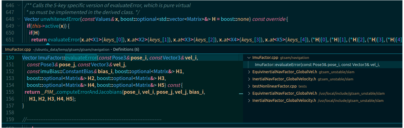
而其中的unwhitenedError函数,则是计算残差和雅可比矩阵的函数,该函数最终调用imu预积分类PreintegratedImuMeasurements中的残差计算,雅可比矩阵求导函数computeErrorAndJacobians。
本文内容由网友自发贡献,版权归原作者所有,本站不承担相应法律责任。如您发现有涉嫌抄袭侵权的内容,请联系:hwhale#tublm.com(使用前将#替换为@)

 至此,摸索清楚了从优化器到残差,雅可比矩阵计算的整个计算流程。