LQR控制倒立摆:
倒立摆状态方程:
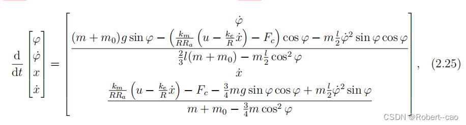
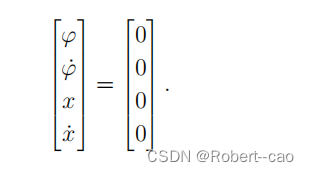
目标任务:
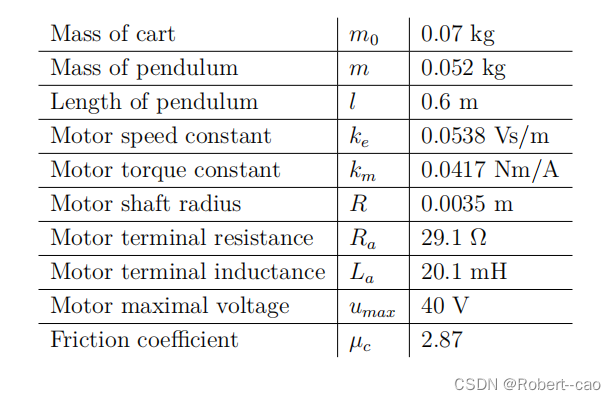
模型参数:
%% LQR for the cart-pole system

load('cp_params.mat');
syms phi phid x xd I u
fr(1) = 0.2;              % friction magnitude
Ts = 0.01;
Duration = 2.5;
Q = [100 0 1 0];          % LQ weights
R = 0.0001;

q1 = [phi; phid; x; xd];
q1 = cp_dynmodel(q1,u,par,fr);

Asym = jacobian(q1,[phi;phid;x;xd]);
A = double(subs(Asym,[phi;phid;x;xd;u],[0;0;0;0;0]));
Bsym = jacobian(q1,u);
B = double(subs(Bsym,[phi;phid;x;xd;u],[0;0;0;0;0]));
A = eye(4)+Ts*A;
B = Ts*B;
clear phi phid x xd I u k1 k2 k3 k4 q1

%% LQR
C = diag([1,1,1,1]);
D = zeros(4,1);
K = dlqr(A,B,diag(Q),R);

%% Simulation
qLQR = zeros(5,Duration/Ts+1);
q = [0.2;0;0;0];
qLQR(:,1) = [q; 0];
for i = 1 : Duration/Ts
    u = -K*q;
    [~,q] = ode45(@(t,q) cp_dynmodel(q,u,par,fr),[0 Ts/2 Ts],q);
    q = q(3,:)';
    qLQR(:,i+1) = [q; u];
end
%% Plots
plotTraj(qLQR,Ts)
首先非线性模型通过雅可比矩阵线性化:
Asym = jacobian(q1,[phi;phid;x;xd]);
A = double(subs(Asym,[phi;phid;x;xd;u],[0;0;0;0;0]));
Bsym = jacobian(q1,u);
B = double(subs(Bsym,[phi;phid;x;xd;u],[0;0;0;0;0]));
离散化模型:
A = eye(4)+Ts*A;
B = Ts*B;
通过LQR计算出反馈矩阵K值:
K = dlqr(A,B,diag(Q),R);
仿真,通过
%% Simulation
qLQR = zeros(5,Duration/Ts+1);
q = [0.2;0;0;0];
qLQR(:,1) = [q; 0];
for i = 1 : Duration/Ts
    u = -K*q;
    [~,q] = ode45(@(t,q) cp_dynmodel(q,u,par,fr),[0 Ts/2 Ts],q);
    q = q(3,:)';
    qLQR(:,i+1) = [q; u];
end
%% Plots
plotTraj(qLQR,Ts)
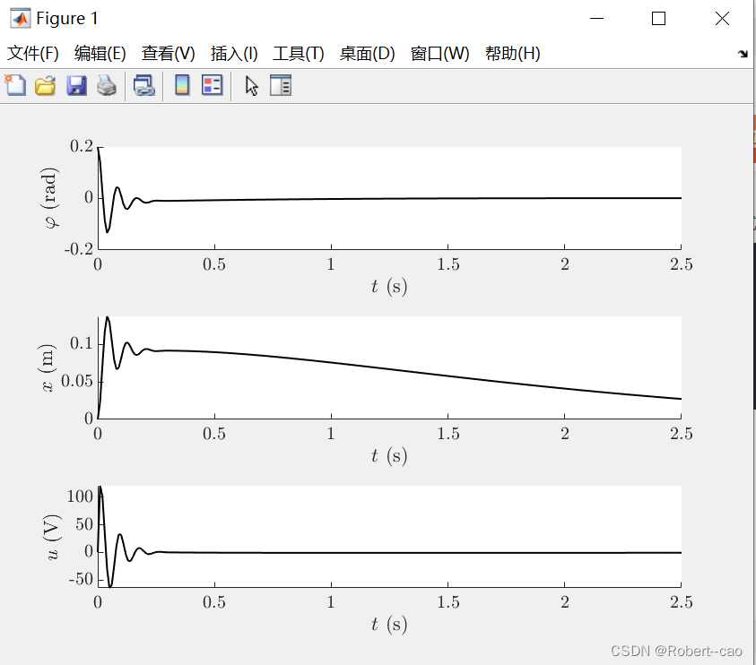
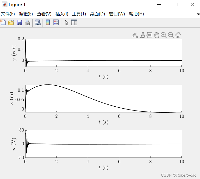
结果:
LQR-MPC控制倒立摆:
这里就是使用mpc产生输入补偿LQR输入:
 input = fmincon(@(u) cost_func_lin(u,horizon,q,Q,R,A2,B),input,[],...
        [],[],[],(K*q-40)*ones(horizon,1),(K*q+40)*ones(horizon,1),[],options);
    u = -K*q + input(1);
%% MPC for the cart-pole system

load('cp_params.mat');
syms phi phid x xd I u
fr(1) = 0.2;              % friction magnitude
Ts = 0.01;
horizon = 25;
Duration = 10;
Q = [100 0 1 0];          % MPC weights
R = 0.0001;

q1 = [phi; phid; x; xd];
q1 = cp_dynmodel(q1,u,par,fr);

Asym = jacobian(q1,[phi;phid;x;xd]);
A = double(subs(Asym,[phi;phid;x;xd;u],[0;0;0;0;0]));
Bsym = jacobian(q1,u);
B = double(subs(Bsym,[phi;phid;x;xd;u],[0;0;0;0;0]));
A = eye(4)+Ts*A;
B = Ts*B; %离散化
clear phi phid x xd I u k1 k2 k3 k4 q1

%% LQ feedback gain
C = diag([1,1,1,1]);
D = zeros(4,1);
K = dlqr(A,B,diag(Q),R);

%% Simulation
A2 = A-B*K;
u = 0;
qlinMPC = zeros(5,Duration/Ts+1);
q = [0.2; 0; 0; 0];        % initial condition
qlinMPC(:,1) = [q; u];
input = zeros(horizon,1);
options = optimoptions('fmincon','Algorithm','sqp');

for i = 1: Duration / Ts
    input = fmincon(@(u) cost_func_lin(u,horizon,q,Q,R,A2,B),input,[],...
        [],[],[],(K*q-40)*ones(horizon,1),(K*q+40)*ones(horizon,1),[],options);
    u = -K*q + input(1);
    [~,q] = ode45(@(t,q) cp_dynmodel(q,u,par,fr),[0 Ts/2 Ts],q);
    q = q(3,:)';
    qlinMPC(:,i+1) = [q; u];
end


%% Plots
plotTraj(qlinMPC,Ts)
关于GPR参考资料:
Gaussian process 的重要组成部分——关于那个被广泛应用的Kernel的林林总总 - 知乎
Documentation for GPML Matlab Code
%% GPMPC for cart-pole dynamic system
addpath '..\TDK_2020\gp' % write path of the containing folder
addpath '..\TDK_2020\util'
load('cp_params.mat');
load('cp_trainingpoints.mat');
fr(1) = 0.2;
Ts = 0.01;
horizon = 25;
Duration = 2.5;
Q = [100 0 1 0];
R = 0.0001;
%% GP training
gpmodel.inputs = xtrain';
gpmodel.targets = ytrain';
[gpmodel2, nlml] = train(gpmodel, 1, 100);
%% Precomputation of GP matrices and vectors
N = length(xtrain(1,:));
L = zeros(4,4,4);
Kxx = zeros(N,N,4);
Kinv = Kxx;
alpha = zeros(N,1,4);
sf = 0.1;
sn = 0.01;
for k = 1:4
L(:,:,k) = diag(1./exp(2*gpmodel2.hyp(1:4,k)));
for i=1:N
for j=1:N
Kxx(i,j,k)=sf^2*kernel(xtrain(:,i),xtrain(:,j),L(:,:,k));
end
end
alpha(:,:,k) = (Kxx(:,:,k)+sn^2*eye(N))\ytrain(k,:)';
Kinv(:,:,k) = inv(Kxx(:,:,k)+sn^2*eye(N));
end
%% Discretisation, linearisation
syms phi phid x xd I u
q1 = [phi; phid; x; xd];
q1 = cp_dynmodel(q1,u,par,fr);
Asym = jacobian(q1,[phi;phid;x;xd]);
A = double(subs(Asym,[phi;phid;x;xd;u],[0;0;0;0;0]));
Bsym = jacobian(q1,u);
B = double(subs(Bsym,[phi;phid;x;xd;u],[0;0;0;0;0]));
A = eye(4)+Ts*A;
B = Ts*B;
clear phi phid x xd I u k1 k2 k3 k4 q1
%% LQR
C = diag([1,1,1,1]);
D = zeros(4,1);
K = dlqr(A,B,diag(Q),R);
%% GPMPC Simulation
A2 = A-B*K;
q = [0.2; 0; 0; 0]; % initial condition
qGPMPC = zeros(5,Duration/Ts+1);
qGPMPC(1:4,1) = q;
input = zeros(horizon,1);
options = optimoptions('fmincon','Algorithm','sqp');
for i = 1: Duration / Ts
input = fmincon(@(u) cost_func_GP(u,horizon,q,Q,R,A2,B,xtrain,L,alpha,Kinv),...
input,[],[],[],[],(K*q-40)*ones(horizon,1),(K*q+40)*ones(horizon,1),[],options);
u = -K*q + input(1);
[~,q] = ode45(@(t,q) cp_dynmodel(q,u,par,fr),[0 Ts/2 Ts],q);
q = q(3,:)';
qGPMPC(:,i+1) = [q; u];
end
%% Plots
plotTraj(qGPMPC,Ts)
%% Plot the prediction at a certain time instant and the simulation
% results at that time interval
niter = horizon;
start = 12; % t = 0.12 s
mean = zeros(4,niter+1);
mean(:,1) = qGPMPC(1:4,start);
u = qGPMPC(5,start);
Ktest = zeros(1,length(xtrain(1,:)));
M = zeros(4,niter);
S = M;
N = length(xtrain(1,:));
for iter = 1:niter
for k = 1:4
for j=1:N
Ktest(1,j,k)=sf^2*kernel(mean(:,iter),xtrain(:,j),L(:,:,k));
end
M(k,iter) = Ktest(:,:,k)*alpha(:,:,k);
S(k,iter) = sf^2 - Ktest(:,:,k)*Kinv(:,:,k)*Ktest(:,:,k)';
end
mean(:,iter+1) = A*mean(:,iter) + B*u + M(:,iter);
end
tsimu = start*Ts:Ts:(start+horizon-1)*Ts;
figure()
subplot(2,1,1)
hold on
plot(tsimu,qGPMPC(1,start:start+niter-1),'r','LineWidth',1)
errorbar(tsimu,mean(1,1:25),2*sqrt(S(1,:)),'k','LineWidth',1)
xlabel('$t$ (s)')
ylabel('$\varphi$ (rad)')
legend('Simulation result','Prediction at $t=0.12$ s')
hold off
subplot(2,1,2)
hold on
plot(tsimu,qGPMPC(3,start:start+niter-1),'r','LineWidth',1)
errorbar(tsimu,mean(3,1:25),2*sqrt(S(3,:)),'k','LineWidth',1)
xlabel('$t$ (s)')
ylabel('$x$ (m)')
hold off
具体代码:
MPC/LQR. LQR-MPC.GP-MPC.rar at main · caokaifa/MPC · GitHub
本文内容由网友自发贡献,版权归原作者所有,本站不承担相应法律责任。如您发现有涉嫌抄袭侵权的内容,请联系:hwhale#tublm.com(使用前将#替换为@)