本节目标:学习gtsam与isam在二位位姿pose2和三维位姿pose3上的使用,并将isam用于位姿的因子图优化。
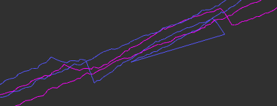
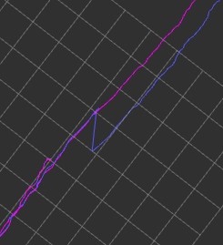
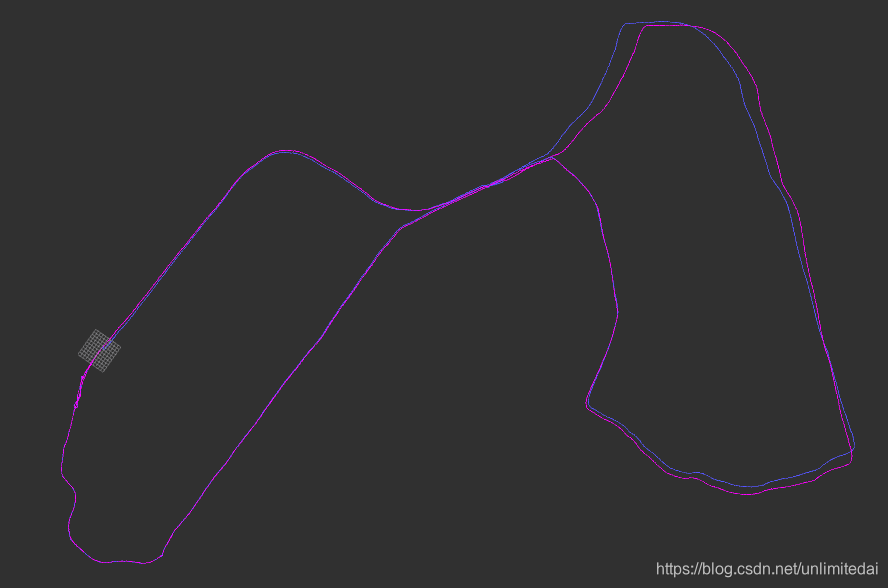
预期效果:将ICP匹配带来的瞬间位移变成对之前累积误差的消除。蓝色ICP无图优化,紫色ICP后进行图优化。

程序:https://gitee.com/eminbogen/one_liom
test_gtsam里有学习 gtsam,isam的四个程序
目录
图优化学习
图优化和因子图优化的简介
gtsam对于二维位姿的使用
isam对于二维位姿的使用
gtsam对于三维位姿的使用
isam对于三维位姿的使用
GPS因子加入
因子图优化用于SLAM
添加内容
示意
图优化学习
图优化和因子图优化的简介
干货:因子图优化的资源合集
深入理解图优化与g2o:图优化篇
iSAM2 笔记
简单来说就是图优化是一次获取所有位姿信息进行优化,因子图优化是逐帧获取逐帧优化,实时且只优化关联帧的位姿信息。
gtsam对于二维位姿的使用
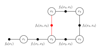
二维优化目标为优化所有x的位姿。
1.定义需要优化的图和优化的参数
NonlinearFactorGraph graph;
Values initials;
2.加入欲优化的初值,添加单点的先验因子,边因子
initials.insert(Symbol('x', 1), Pose2(0.2, -0.3, 0.2));
initials.insert(Symbol('x', 2), Pose2(5.1, 0.3, -0.1));
initials.insert(Symbol('x', 3), Pose2(9.9, -0.1, -M_PI_2 - 0.2));
initials.insert(Symbol('x', 4), Pose2(10.2, -5.0, -M_PI + 0.1));
initials.insert(Symbol('x', 5), Pose2(5.1, -5.1, M_PI_2 - 0.1));
graph.add(PriorFactor<Pose2>(Symbol('x', 1), Pose2(0, 0, 0), priorModel));
graph.add(BetweenFactor<Pose2>(Symbol('x', 1), Symbol('x', 2), Pose2(5, 0, 0), odomModel));
graph.add(BetweenFactor<Pose2>(Symbol('x', 2), Symbol('x', 3), Pose2(5, 0, -M_PI_2), odomModel));
graph.add(BetweenFactor<Pose2>(Symbol('x', 3), Symbol('x', 4), Pose2(5, 0, -M_PI_2), odomModel));
graph.add(BetweenFactor<Pose2>(Symbol('x', 4), Symbol('x', 5), Pose2(5, 0, -M_PI_2), odomModel));
3.设置gtsam参数,并将参数输入gtsam优化函数
GaussNewtonParams parameters;
parameters.setVerbosity("ERROR");
parameters.setMaxIterations(20);
parameters.setLinearSolverType("MULTIFRONTAL_QR");
4.进行图优化,获取优化结果
GaussNewtonOptimizer optimizer(graph, initials, parameters);
Values results = optimizer.optimize();
整体程序来源于官方文档:
#include <gtsam/geometry/Pose2.h>
#include <gtsam/nonlinear/NonlinearFactorGraph.h>
#include <gtsam/nonlinear/Values.h>
#include <gtsam/inference/Symbol.h>
#include <gtsam/slam/PriorFactor.h>
#include <gtsam/slam/BetweenFactor.h>
#include <gtsam/nonlinear/GaussNewtonOptimizer.h>
#include <gtsam/nonlinear/Marginals.h>
using namespace std;
using namespace gtsam;
int main(int argc, char** argv)
{
    NonlinearFactorGraph graph;

    Values initials;
    initials.insert(Symbol('x', 1), Pose2(0.2, -0.3, 0.2));
    initials.insert(Symbol('x', 2), Pose2(5.1, 0.3, -0.1));
    initials.insert(Symbol('x', 3), Pose2(9.9, -0.1, -M_PI_2 - 0.2));
    initials.insert(Symbol('x', 4), Pose2(10.2, -5.0, -M_PI + 0.1));
    initials.insert(Symbol('x', 5), Pose2(5.1, -5.1, M_PI_2 - 0.1));
    initials.print("\nInitial Values:\n");
    //固定第一个顶点,在gtsam中相当于添加一个先验因子
    noiseModel::Diagonal::shared_ptr priorModel = noiseModel::Diagonal::Sigmas(Vector3(1.0, 1.0, 0.1));
    graph.add(PriorFactor<Pose2>(Symbol('x', 1), Pose2(0, 0, 0), priorModel));

    //二元位姿因子
    noiseModel::Diagonal::shared_ptr odomModel = noiseModel::Diagonal::Sigmas(Vector3(0.5, 0.5, 0.1));
    graph.add(BetweenFactor<Pose2>(Symbol('x', 1), Symbol('x', 2), Pose2(5, 0, 0), odomModel));
    graph.add(BetweenFactor<Pose2>(Symbol('x', 2), Symbol('x', 3), Pose2(5, 0, -M_PI_2), odomModel));
    graph.add(BetweenFactor<Pose2>(Symbol('x', 3), Symbol('x', 4), Pose2(5, 0, -M_PI_2), odomModel));
    graph.add(BetweenFactor<Pose2>(Symbol('x', 4), Symbol('x', 5), Pose2(5, 0, -M_PI_2), odomModel));

    //二元回环因子
    noiseModel::Diagonal::shared_ptr loopModel = noiseModel::Diagonal::Sigmas(Vector3(0.5, 0.5, 0.1));
    graph.add(BetweenFactor<Pose2>(Symbol('x', 5), Symbol('x', 2), Pose2(5, 0, -M_PI_2), loopModel));
    graph.print("\nFactor Graph:\n");


    GaussNewtonParams parameters;
    parameters.setVerbosity("ERROR");
    parameters.setMaxIterations(20);
    parameters.setLinearSolverType("MULTIFRONTAL_QR");
    GaussNewtonOptimizer optimizer(graph, initials, parameters);
    Values results = optimizer.optimize();
    results.print("Final Result:\n");

    Marginals marginals(graph, results);
    cout << "x1 covariance:\n" << marginals.marginalCovariance(Symbol('x', 1)) << endl;
    cout << "x2 covariance:\n" << marginals.marginalCovariance(Symbol('x', 2)) << endl;
    cout << "x3 covariance:\n" << marginals.marginalCovariance(Symbol('x', 3)) << endl;
    cout << "x4 covariance:\n" << marginals.marginalCovariance(Symbol('x', 4)) << endl;
    cout << "x5 covariance:\n" << marginals.marginalCovariance(Symbol('x', 5)) << endl;

    return 0;
}
效果:
isam对于二维位姿的使用
1.定义需要优化的图和优化的参数
NonlinearFactorGraph graph;
Values initialEstimate;
2.加入欲优化的初值,添加单点的先验因子,边因子
initPose.push_back(Pose2(0.5, 0.0,  0.2   ));
initialEstimate.insert(i+1, initPose[i]);
......
graph.push_back(PriorFactor<Pose2>(1, Pose2(0, 0, 0), priorNoise));
......
gra.push_back(BetweenFactor<Pose2>(1, 2, Pose2(2, 0, 0     ), model));
graph.push_back(BetweenFactor<Pose2>(1, 2, Pose2(2, 0, 0     ), model));
......
3.设置iSAM参数,并将参数输入ISAM优化函数
ISAM2Params parameters;
parameters.relinearizeThreshold = 0.01;
parameters.relinearizeSkip = 1;
ISAM2 isam(parameters);
4.每次或多次加入后进行因子图优化
isam.update(graph, initialEstimate);
isam.update();
全部程序来源于博客《isam2 优化pose graph》
#include <gtsam/inference/Symbol.h>
#include <gtsam/nonlinear/ISAM2.h>
#include <gtsam/nonlinear/NonlinearFactorGraph.h>
#include <gtsam/nonlinear/Values.h>
#include <vector>
#include <gtsam/geometry/Pose2.h>
#include <gtsam/inference/Key.h>
#include <gtsam/slam/PriorFactor.h>
#include <gtsam/slam/BetweenFactor.h>
#include <gtsam/nonlinear/Values.h>

using namespace std;
using namespace gtsam;

int main()
{

  // 向量保存好模拟的位姿和测量,到时候一个个往isam2里填加
  std::vector< BetweenFactor<Pose2> > gra;
  std::vector< Pose2 > initPose;

  noiseModel::Diagonal::shared_ptr model = noiseModel::Diagonal::Sigmas(Vector3(0.2, 0.2, 0.1));

  gra.push_back(BetweenFactor<Pose2>(1, 2, Pose2(2, 0, 0     ), model));
  gra.push_back(BetweenFactor<Pose2>(2, 3, Pose2(2, 0, M_PI_2), model));
  gra.push_back(BetweenFactor<Pose2>(3, 4, Pose2(2, 0, M_PI_2), model));
  gra.push_back(BetweenFactor<Pose2>(4, 5, Pose2(2, 0, M_PI_2), model));
  gra.push_back(BetweenFactor<Pose2>(5, 2, Pose2(2, 0, M_PI_2), model));

  initPose.push_back(Pose2(0.5, 0.0,  0.2   ));
  initPose.push_back( Pose2(2.3, 0.1, -0.2   ));
  initPose.push_back( Pose2(4.1, 0.1,  M_PI_2));
  initPose.push_back( Pose2(4.0, 2.0,  M_PI  ));
  initPose.push_back( Pose2(2.1, 2.1, -M_PI_2));

  ISAM2Params parameters;
  parameters.relinearizeThreshold = 0.01;
  parameters.relinearizeSkip = 1;
  ISAM2 isam(parameters);

  // 注意isam2的graph里只添加isam2更新状态以后新测量到的约束
  NonlinearFactorGraph graph;
  Values initialEstimate;

  // the first pose don't need to update
  for( int i =0; i<5 ;i++)
  {
          // Add an initial guess for the current pose
           initialEstimate.insert(i+1, initPose[i]);

           if(i == 0)
           {
               //  Add a prior on the first pose, setting it to the origin
               // A prior factor consists of a mean and a noise model (covariance matrix)
               noiseModel::Diagonal::shared_ptr priorNoise = noiseModel::Diagonal::Sigmas(Vector3(0.3, 0.3, 0.1));
               graph.push_back(PriorFactor<Pose2>(1, Pose2(0, 0, 0), priorNoise));

           }else
           {

               graph.push_back(gra[i-1]);  // ie: when i = 1 , robot at pos2,  there is a edge gra[0] between pos1 and pos2
               if(i == 4)
               {
                   graph.push_back(gra[4]);  //  when robot at pos5, there two edge, one is pos4 ->pos5, another is pos5->pos2  (grad[4])
               }
               isam.update(graph, initialEstimate);
               isam.update();

               Values currentEstimate = isam.calculateEstimate();
               cout << "****************************************************" << endl;
               cout << "Frame " << i << ": " << endl;
               currentEstimate.print("Current estimate: ");

               // Clear the factor graph and values for the next iteration
               // 特别重要,update以后,清空原来的约束。已经加入到isam2的那些会用bayes tree保管,你不用操心了。
               graph.resize(0);
               initialEstimate.clear();
           }
  }
  return 0;
}
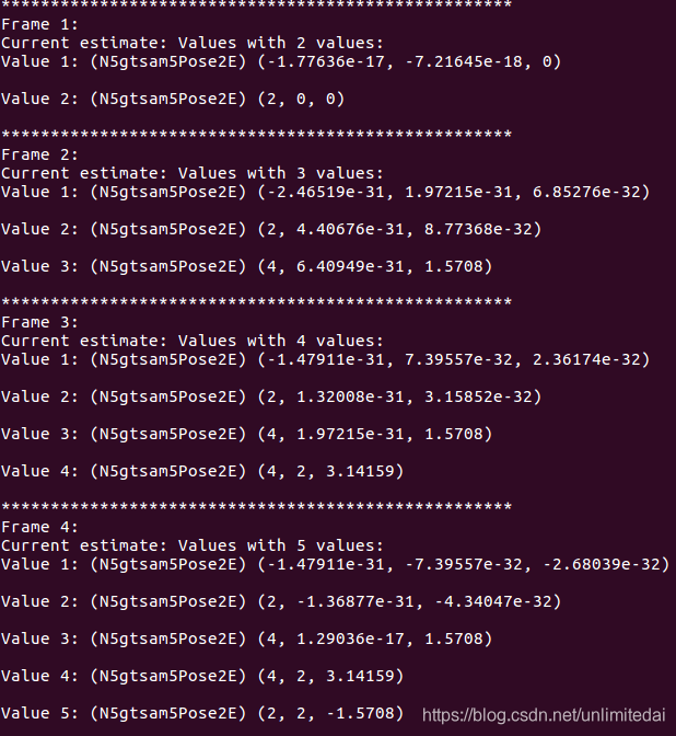
效果就是逐帧的。
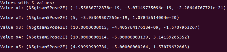
gtsam对于三维位姿的使用
对于三维位姿我们优化如下位姿数据的图。
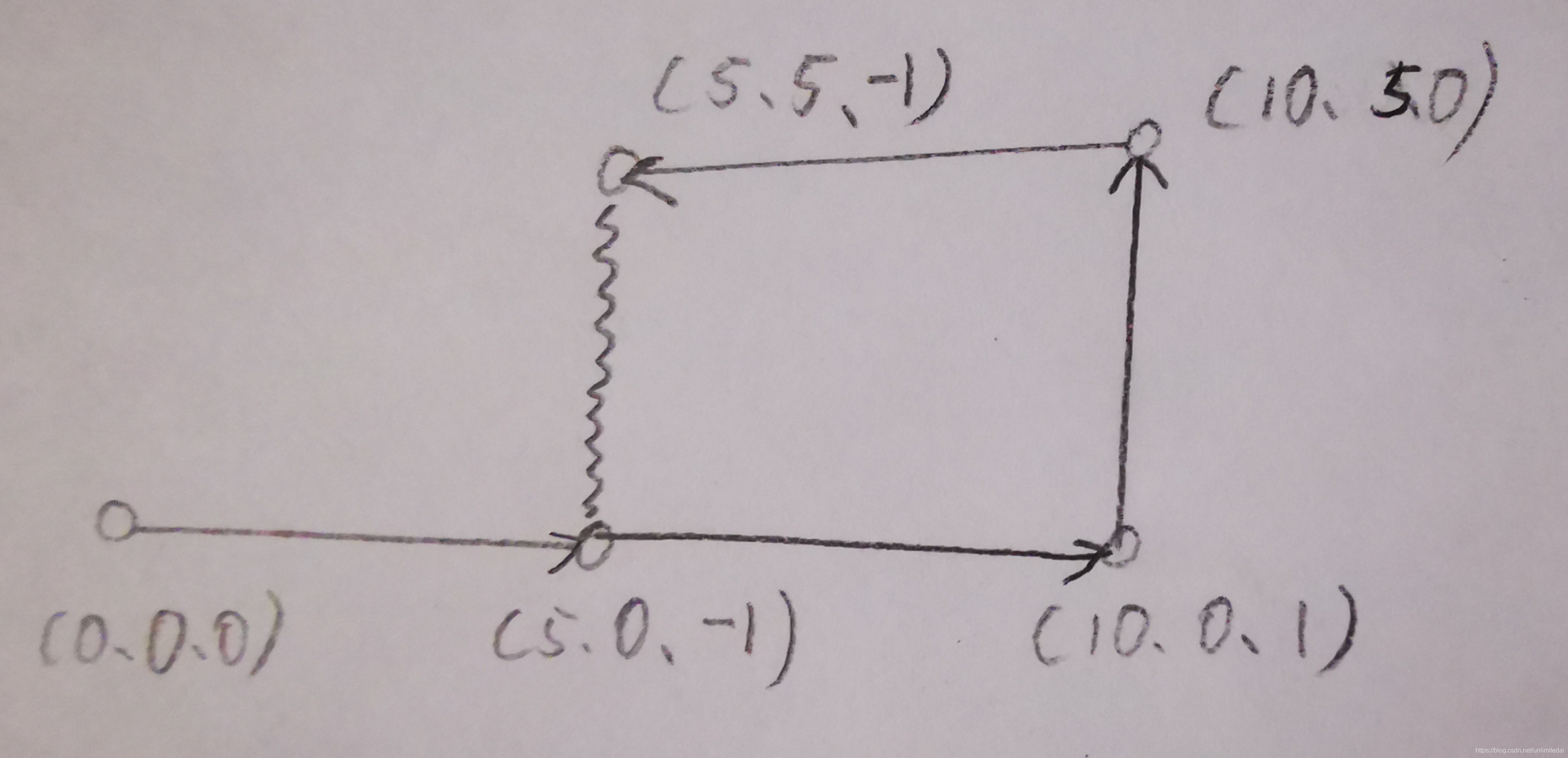
与二维位姿不同,三维位姿要使用pose3,由欧拉角和t组成,只改变第二步即可。
1.定义需要优化的图和优化的参数
NonlinearFactorGraph graph;
Values initials;
2.加入欲优化的初值,添加单点的先验因子,边因子
initials.insert(Symbol('x', 1), Pose3(Rot3::RzRyRx(0, 0, 0), Point3(0.1, -0.1, 0)));
initials.insert(Symbol('x', 2), Pose3(Rot3::RzRyRx(0, 0, 0), Point3(6, 0.1, -1.1)));
initials.insert(Symbol('x', 3), Pose3(Rot3::RzRyRx(0, 0, 0), Point3(10.1, -0.1, 0.9)));
initials.insert(Symbol('x', 4), Pose3(Rot3::RzRyRx(0, 0, 0), Point3(10, 5, 0)));
initials.insert(Symbol('x', 5), Pose3(Rot3::RzRyRx(0, 0, 0), Point3(5.1, 4.9, -0.9)));
graph.add(PriorFactor<Pose3>(Symbol('x', 1), Pose3(Rot3::RzRyRx(0, 0, 0), Point3(0, 0, 0)), priorNoise));
graph.add(BetweenFactor<Pose3>(Symbol('x', 1), Symbol('x', 2), Pose3(Rot3::RzRyRx(0, 0, 0), Point3(5, 0, -1)), odometryNoise));
graph.add(BetweenFactor<Pose3>(Symbol('x', 2), Symbol('x', 3), Pose3(Rot3::RzRyRx(0, 0, 0), Point3(5, 0, 2)), odometryNoise));
graph.add(BetweenFactor<Pose3>(Symbol('x', 3), Symbol('x', 4), Pose3(Rot3::RzRyRx(0, 0, 0), Point3(0, 5, -1)), odometryNoise));
graph.add(BetweenFactor<Pose3>(Symbol('x', 4), Symbol('x', 5), Pose3(Rot3::RzRyRx(0, 0, 0), Point3(-5, 0, -1)), odometryNoise));
3.设置gtsam参数,并将参数输入gtsam优化函数
GaussNewtonParams parameters;
parameters.setVerbosity("ERROR");
parameters.setMaxIterations(20);
parameters.setLinearSolverType("MULTIFRONTAL_QR");
4.进行图优化,获取优化结果
GaussNewtonOptimizer optimizer(graph, initials, parameters);
Values results = optimizer.optimize();
整体程序:
#include <gtsam/geometry/Rot3.h>
#include <gtsam/geometry/Pose3.h>
#include <gtsam/nonlinear/NonlinearFactorGraph.h>
#include <gtsam/nonlinear/Values.h>
#include <gtsam/inference/Symbol.h>
#include <gtsam/slam/PriorFactor.h>
#include <gtsam/slam/BetweenFactor.h>
#include <gtsam/nonlinear/GaussNewtonOptimizer.h>
#include <gtsam/nonlinear/Marginals.h>
using namespace std;
using namespace gtsam;
int main(int argc, char** argv)
{
    NonlinearFactorGraph graph;

    Values initials;
    initials.insert(Symbol('x', 1), Pose3(Rot3::RzRyRx(0, 0, 0), Point3(0.1, -0.1, 0)));
    initials.insert(Symbol('x', 2), Pose3(Rot3::RzRyRx(0, 0, 0), Point3(6, 0.1, -1.1)));
    initials.insert(Symbol('x', 3), Pose3(Rot3::RzRyRx(0, 0, 0), Point3(10.1, -0.1, 0.9)));
    initials.insert(Symbol('x', 4), Pose3(Rot3::RzRyRx(0, 0, 0), Point3(10, 5, 0)));
    initials.insert(Symbol('x', 5), Pose3(Rot3::RzRyRx(0, 0, 0), Point3(5.1, 4.9, -0.9)));
    initials.print("\nInitial Values:\n");
    //固定第一个顶点,在gtsam中相当于添加一个先验因子
    noiseModel::Diagonal::shared_ptr priorNoise = noiseModel::Diagonal::Variances(
          (Vector(6) << 1e-2, 1e-2, M_PI * M_PI, 1e8, 1e8, 1e8).finished());
    graph.add(PriorFactor<Pose3>(Symbol('x', 1), Pose3(Rot3::RzRyRx(0, 0, 0), Point3(0, 0, 0)), priorNoise));

    //二元位姿因子
    noiseModel::Diagonal::shared_ptr odometryNoise = noiseModel::Diagonal::Variances(
          (Vector(6) << 1e-6, 1e-6, 1e-6, 1e-4, 1e-4, 1e-4).finished());
    graph.add(BetweenFactor<Pose3>(Symbol('x', 1), Symbol('x', 2), Pose3(Rot3::RzRyRx(0, 0, 0), Point3(5, 0, -1)), odometryNoise));
    graph.add(BetweenFactor<Pose3>(Symbol('x', 2), Symbol('x', 3), Pose3(Rot3::RzRyRx(0, 0, 0), Point3(5, 0, 2)), odometryNoise));
    graph.add(BetweenFactor<Pose3>(Symbol('x', 3), Symbol('x', 4), Pose3(Rot3::RzRyRx(0, 0, 0), Point3(0, 5, -1)), odometryNoise));
    graph.add(BetweenFactor<Pose3>(Symbol('x', 4), Symbol('x', 5), Pose3(Rot3::RzRyRx(0, 0, 0), Point3(-5, 0, -1)), odometryNoise));

    //二元回环因子
    noiseModel::Diagonal::shared_ptr loopModel = noiseModel::Diagonal::Variances(
          (Vector(6) << 1e-6, 1e-6, 1e-6, 1e-4, 1e-4, 1e-4).finished());
    graph.add(BetweenFactor<Pose3>(Symbol('x', 5), Symbol('x', 2), Pose3(Rot3::RzRyRx(0, 0, 0), Point3(0, -5, 0)), loopModel));
    graph.print("\nFactor Graph:\n");


    GaussNewtonParams parameters;
    parameters.setVerbosity("ERROR");
    parameters.setMaxIterations(20);
    parameters.setLinearSolverType("MULTIFRONTAL_QR");
    GaussNewtonOptimizer optimizer(graph, initials, parameters);
    Values results = optimizer.optimize();
    results.print("Final Result:\n");

    Marginals marginals(graph, results);
    cout << "x1 covariance:\n" << marginals.marginalCovariance(Symbol('x', 1)) << endl;
    cout << "x2 covariance:\n" << marginals.marginalCovariance(Symbol('x', 2)) << endl;
    cout << "x3 covariance:\n" << marginals.marginalCovariance(Symbol('x', 3)) << endl;
    cout << "x4 covariance:\n" << marginals.marginalCovariance(Symbol('x', 4)) << endl;
    cout << "x5 covariance:\n" << marginals.marginalCovariance(Symbol('x', 5)) << endl;

    return 0;
}
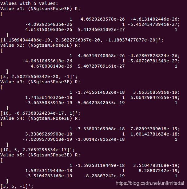
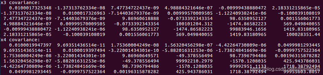
效果有旋转矩阵和t,协方差为6*6的,应该是t的xyz和欧拉角rpy。
isam对于三维位姿的使用
同样只有第二步修改。
1.定义需要优化的图和优化的参数
NonlinearFactorGraph graph;
Values initialEstimate;
2.加入欲优化的初值,添加单点的先验因子,边因子
initPose.push_back( Pose3(Rot3::RzRyRx(0, 0, 0), Point3(0.1, -0.1, 0)));
initialEstimate.insert(i+1, initPose[i]);
......
graph.push_back(PriorFactor<Pose3>(1, Pose3(Rot3::RzRyRx(0, 0, 0), Point3(0, 0, 0)), priorNoise));
......
gra.push_back(BetweenFactor<Pose3>(1, 2, Pose3(Rot3::RzRyRx(0, 0, 0), Point3(5, 0, -1)), model));
graph.push_back(BetweenFactor<Pose2>(1, 2, Pose2(2, 0, 0     ), model));
......
3.设置iSAM参数,并将参数输入ISAM优化函数
ISAM2Params parameters;
parameters.relinearizeThreshold = 0.01;
parameters.relinearizeSkip = 1;
ISAM2 isam(parameters);
4.每次或多次加入后进行因子图优化
isam.update(graph, initialEstimate);
isam.update();
全部程序:
#include <gtsam/inference/Symbol.h>
#include <gtsam/nonlinear/ISAM2.h>
#include <gtsam/nonlinear/NonlinearFactorGraph.h>
#include <gtsam/nonlinear/Values.h>
#include <vector>
#include <gtsam/inference/Key.h>
#include <gtsam/slam/PriorFactor.h>
#include <gtsam/slam/BetweenFactor.h>
#include <gtsam/nonlinear/Values.h>
#include <gtsam/geometry/Rot3.h>
#include <gtsam/geometry/Pose3.h>

using namespace std;
using namespace gtsam;

int main()
{

  // 向量保存好模拟的位姿和测量,到时候一个个往isam2里填加
  std::vector< BetweenFactor<Pose3> > gra;
  std::vector< Pose3 > initPose;

  // For simplicity, we will use the same noise model for odometry and loop closures
  noiseModel::Diagonal::shared_ptr model = noiseModel::Diagonal::Variances(
          (Vector(6) << 1e-6, 1e-6, 1e-6, 1e-4, 1e-4, 1e-4).finished());

  gra.push_back(BetweenFactor<Pose3>(1, 2, Pose3(Rot3::RzRyRx(0, 0, 0), Point3(5, 0, -1)), model));
  gra.push_back(BetweenFactor<Pose3>(2, 3, Pose3(Rot3::RzRyRx(0, 0, 0), Point3(5, 0, 2)), model));
  gra.push_back(BetweenFactor<Pose3>(3, 4, Pose3(Rot3::RzRyRx(0, 0, 0), Point3(0, 5, -1)), model));
  gra.push_back(BetweenFactor<Pose3>(4, 5, Pose3(Rot3::RzRyRx(0, 0, 0), Point3(-5, 0, -1)), model));
  gra.push_back(BetweenFactor<Pose3>(5, 2, Pose3(Rot3::RzRyRx(0, 0, 0), Point3(0, -5, 0)), model));

  initPose.push_back( Pose3(Rot3::RzRyRx(0, 0, 0), Point3(0.1, -0.1, 0)));
  initPose.push_back( Pose3(Rot3::RzRyRx(0, 0, 0), Point3(6, 0.1, -1.1)));
  initPose.push_back( Pose3(Rot3::RzRyRx(0, 0, 0), Point3(10.1, -0.1, 0.9)));
  initPose.push_back( Pose3(Rot3::RzRyRx(0, 0, 0), Point3(10, 5, 0)));
  initPose.push_back( Pose3(Rot3::RzRyRx(0, 0, 0), Point3(5.1, 4.9, -0.9)));

  ISAM2Params parameters;
  parameters.relinearizeThreshold = 0.01;
  parameters.relinearizeSkip = 1;
  ISAM2 isam(parameters);

  NonlinearFactorGraph graph;
  Values initialEstimate;

  for( int i =0; i<5 ;i++)
  {
           initialEstimate.insert(i+1, initPose[i]);

           if(i == 0)
           {
               noiseModel::Diagonal::shared_ptr priorNoise = noiseModel::Diagonal::Variances(
		(Vector(6) << 1e-2, 1e-2, M_PI * M_PI, 1e8, 1e8, 1e8).finished());
               graph.push_back(PriorFactor<Pose3>(1, Pose3(Rot3::RzRyRx(0, 0, 0), Point3(0, 0, 0)), priorNoise));

           }else
           {

               graph.push_back(gra[i-1]);  // ie: when i = 1 , robot at pos2,  there is a edge gra[0] between pos1 and pos2
               if(i == 4)
               {
                   graph.push_back(gra[4]);  //  when robot at pos5, there two edge, one is pos4 ->pos5, another is pos5->pos2  (grad[4])
               }
               isam.update(graph, initialEstimate);
               isam.update();

               Values currentEstimate = isam.calculateEstimate();
               cout << "****************************************************" << endl;
               cout << "Frame " << i << ": " << endl;
               currentEstimate.print("Current estimate: ");

               // Clear the factor graph and values for the next iteration
               // 特别重要,update以后,清空原来的约束。已经加入到isam2的那些会用bayes tree保管,你不用操心了。
               graph.resize(0);
               initialEstimate.clear();
           }
  }
  return 0;
}
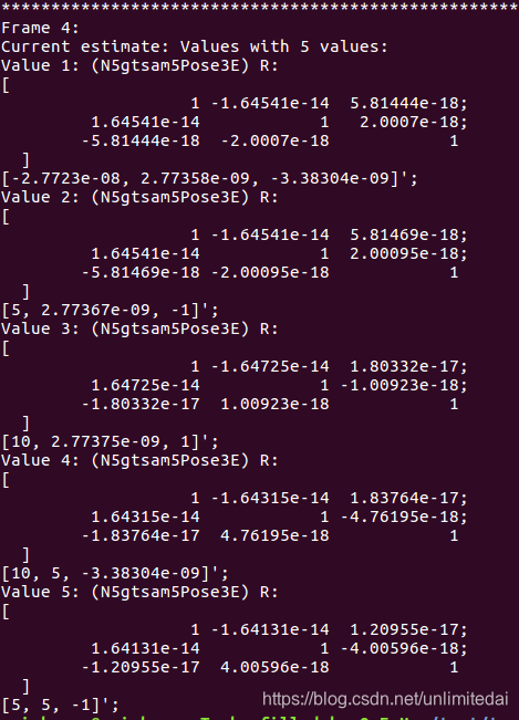
效果:
GPS因子加入
gtsam::GPSFactor gps_factor(Ind, gtsam::Point3(gps_x, gps_y, gps_z), gps_noise);
graph.add(gps_factor);
isam.update(graph, initialEstimate);
因子图优化用于SLAM
添加内容
0.配置文件添加
CMakelist:
find_package(Boost COMPONENTS thread filesystem date_time system REQUIRED)
find_package(GTSAM REQUIRED)
include_directories(
	include
	${Boost_INCLUDE_DIR}
	${GTSAM_INCLUDE_DIR})
add_executable(map src/map.cpp)
target_link_libraries(map ${catkin_LIBRARIES} ${PCL_LIBRARIES} ${CERES_LIBRARIES} ${Boost_LIBRARIES} -lgtsam -ltbb)

package:
<build_depend>GTSAM</build_depend>

头文件:
#include <gtsam/inference/Symbol.h>
#include <gtsam/nonlinear/ISAM2.h>
#include <gtsam/nonlinear/NonlinearFactorGraph.h>
#include <gtsam/nonlinear/Values.h>
#include <gtsam/inference/Key.h>
#include <gtsam/slam/PriorFactor.h>
#include <gtsam/slam/BetweenFactor.h>
#include <gtsam/nonlinear/Values.h>
#include <gtsam/geometry/Rot3.h>
#include <gtsam/geometry/Pose3.h>
1.先验信息
//保存初始点信息,为先验因子。下面操作是把四元数转换为旋转矩阵,旋转矩阵变化为欧拉角
Eigen::Matrix3d rx = q_w_curr.toRotationMatrix();
Eigen::Vector3d ea = rx.eulerAngles(2,1,0);
initialEstimate.insert(temp_laserCloudMap_Ind+1,Pose3(Rot3::RzRyRx(ea[0], ea[1], ea[2]), Point3(t_w_curr.x(), t_w_curr.y(), t_w_curr.z())) );
noiseModel::Diagonal::shared_ptr priorNoise = noiseModel::Diagonal::Variances(
	      (Vector(6) << 1e-2, 1e-2, M_PI * M_PI, 1e8, 1e8, 1e8).finished());
graph.add(PriorFactor<Pose3>(1, Pose3(Rot3::RzRyRx(0, 0, 0), Point3(0, 0, 0)), priorNoise));
2.当前帧信息和里程计变换信息
//保存当前位姿和里程计变换的信息到gtsam的graph,
Eigen::Matrix3d rx_last = q_w_last.toRotationMatrix();
Eigen::Vector3d ea_last = rx_last.eulerAngles(2,1,0);
Eigen::Matrix3d rx_curr = q_w_curr.toRotationMatrix();
Eigen::Vector3d ea_curr = rx_curr.eulerAngles(2,1,0);
initialEstimate.insert(temp_laserCloudMap_Ind+1,Pose3(Rot3::RzRyRx(ea_curr[0], ea_curr[1], ea_curr[2]), Point3(t_w_curr.x(), t_w_curr.y(), t_w_curr.z())) );
//gtsam提供一种容易求两点之间位姿变化的函数between,用于里程计变化信息的录入
gtsam::Pose3 poseFrom = Pose3(Rot3::RzRyRx(ea_last[0], ea_last[1], ea_last[2]), Point3(t_w_last.x(), t_w_last.y(), t_w_last.z()));
gtsam::Pose3 poseTo =   Pose3(Rot3::RzRyRx(ea_curr[0], ea_curr[1], ea_curr[2]), Point3(t_w_curr.x(), t_w_curr.y(), t_w_curr.z()));
noiseModel::Diagonal::shared_ptr odom_noise = noiseModel::Diagonal::Variances((Vector(6) << 1e-6, 1e-6, 1e-6, 1e-4, 1e-4, 1e-4).finished());
graph.add(BetweenFactor<Pose3>(temp_laserCloudMap_Ind,temp_laserCloudMap_Ind+1, poseFrom.between(poseTo),odom_noise));
3.闭环信息
//发生闭环,添加闭环信息到gtsam的graph,闭环noise使用icp得分
Values isamCurrentEstimate1;
Pose3 closeEstimate;
isamCurrentEstimate1 = isam.calculateEstimate();
closeEstimate = isamCurrentEstimate1.at<Pose3>(history_close_Ind+1);

Eigen::Matrix3d rx_temp = q_w_temp.toRotationMatrix();
Eigen::Vector3d ea_temp = rx_temp.eulerAngles(2,1,0);
gtsam::Pose3 poseTemp =   Pose3(Rot3::RzRyRx(ea_temp[0], ea_temp[1], ea_temp[2]), Point3(t_w_temp.x(), t_w_temp.y(), t_w_temp.z()));
noiseModel::Diagonal::shared_ptr closure_noise = noiseModel::Diagonal::Variances((Vector(6) << icp_score, icp_score, icp_score, icp_score, icp_score,icp_score).finished());
graph.add(BetweenFactor<Pose3>(history_close_Ind+1,temp_laserCloudMap_Ind+1, closeEstimate.between(poseTemp),closure_noise));
4.优化后路径输出
//输出gtsam优化后的轨迹
nav_msgs::Path laserGtsamPath;
for(int i=0;i<temp_laserCloudMap_Ind;i++)
{
    nav_msgs::Odometry laserGtsamOdometry;
    Pose3 oneEstimate;
    oneEstimate = isamCurrentEstimate2.at<Pose3>(i+1);
    laserGtsamOdometry.header.frame_id = "map";
    laserGtsamOdometry.child_frame_id = "map_child";
    laserGtsamOdometry.header.stamp = all_time[i];
    laserGtsamOdometry.pose.pose.orientation.x = oneEstimate.rotation().toQuaternion().x();
    laserGtsamOdometry.pose.pose.orientation.y = oneEstimate.rotation().toQuaternion().y();
    laserGtsamOdometry.pose.pose.orientation.z = oneEstimate.rotation().toQuaternion().z();
    laserGtsamOdometry.pose.pose.orientation.w = oneEstimate.rotation().toQuaternion().w();
    laserGtsamOdometry.pose.pose.position.x = oneEstimate.translation().x();
    laserGtsamOdometry.pose.pose.position.y = oneEstimate.translation().y();
    laserGtsamOdometry.pose.pose.position.z = oneEstimate.translation().z();

    geometry_msgs::PoseStamped laserGtsamPose;
    laserGtsamPose.header = laserGtsamOdometry.header;
    laserGtsamPose.pose = laserGtsamOdometry.pose.pose;
    laserGtsamPath.header.stamp = laserGtsamOdometry.header.stamp;
    laserGtsamPath.poses.push_back(laserGtsamPose);
    laserGtsamPath.header.frame_id = "map";
    pubLaserGtsamPath.publish(laserGtsamPath);
}
示意
可以看出对于原本位移明显地区有了很好的平滑,且修改是基于全局的累积误差消除进行的。
本文内容由网友自发贡献,版权归原作者所有,本站不承担相应法律责任。如您发现有涉嫌抄袭侵权的内容,请联系:hwhale#tublm.com(使用前将#替换为@)