本项目只是负责把框架搭建起来,没有进行重训练的微调或者去研究应该剪哪里比较好,需要自己去研究
YOLOv4代码参考:Pytorch 搭建自己的YoloV4目标检测平台(Bubbliiiing 深度学习 教程)_哔哩哔哩_bilibili
Paper:Pruning Filters for Efficient ConvNets
文字内容有点多,请耐心看完【当然直接用代码也可以】
目录
安装
导入包
模型的实例化(针对已经训练好的模型)
对于非单层卷积的通道剪枝(不用看3.1)
剪枝之前统计一下模型的参数量
1. setup strategy (L1 Norm) 计算每个通道的权重
2.建立依赖图(与torch.jit很像)
3.分情况(1.单个卷积进行剪枝 2.层进行剪枝)
3.1 单个卷积(会返回要剪枝的通道索引,这个通道是索引是根据L1正则得到的)
3.2 层剪枝(需要筛选出不需要剪枝的层,比如yolo需要把头部的预测部分取出来,这个是不需要剪枝的)
预测部分
代码
对于单层剪枝主要分以下步骤[怕自己翻译有差距,所以各位可自行翻译理解]:
1. For each filter  , calculate the sum of its absolute kernel weights
  .
.
2. Sort the filters by  .
.
3. Prune m filters with the smallest sum values and their corresponding feature maps. The kernels in the next convolutional layer corresponding to the pruned feature maps are also removed.
4. A new kernel matrix is created for both the ith and i + 1th layers, and the remaining kernel weights are copied to the new model.
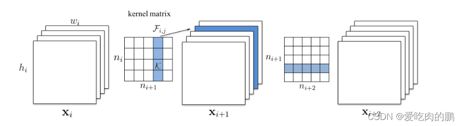
大致意思就说对于你要剪的滤波器(就是卷积了),计算每个通道权重绝对值之和,就是L1,将计算结果进行排序,然后用一个最小值(可以理解为一个阈值)和这些卷积核相关的特征层的m个通道进行剪枝,剪枝以后会生成一个新的卷积核,将原来卷积核内没有被剪的权重赋值给现在得到的新卷积核。
比如你的输入特征层Xi大小为hi,wi,c,c是通道数。卷积核的输入通道数是ni,这个ni=c,输出通道数为ni+1,现在你要在ni+1处剪掉一个通道(图中蓝色部分),我们知道,卷积的时候,输出多少通道,那么下一个特征图Xi+1相应的也会得到相同数量的特征层,现在我们把一个通道移除了,那么相应的,得到的特征层通道数量上也会减少(即Xi+1中蓝色部分会移除)。然后再下一个卷积的输入通道数ni+1又会和Xi+1的通道数一样,所以该卷积核也会减少相应的一个通道维度。对一个卷积进行剪枝,那么就会影响到下一个卷积的维度变化。
单层剪枝
多层剪枝(两种策略):
• Independent pruning determines which filters should be pruned at each layer independent of other layers.
• Greedy pruning accounts for the filters that have been removed in the previous layers. This strategy does not consider the kernels for the previously pruned feature maps while calculating the sum of absolute weights.
1. 独立剪枝:对每一层的滤波器(卷积核)决定是否剪枝与其他层无关
2.贪婪剪枝:考虑先前层中所移除的滤波器。在剪枝计算权重绝对值之和时,不需要考虑先前已剪枝的特征图所对应的核
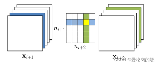
对于策略1独立剪枝,核的绿色部分是计算输出通道绝对值之和时,不考虑之前移除的特征层的这一维度(蓝色部分),也就是只考虑绿色这一列通道之和(这里的个人理解:蓝色这一行在单层剪枝是直接去掉的,也就是图中黄色部分都没有了,但在多层的独立剪枝中,在ni+2方向上只把蓝色区域去除,但黄色的部分要保留),所以核内黄色区域权重保留!
在策略2的贪婪剪枝中,不去统计在特征层中准备剪掉的通道[即考虑先前层中移除的]【个人理解,就是这里又不考虑黄色部分了吧】【可以自己翻译理解下:The greedy pruning strategy does not count kernels for the already pruned feature maps.】
多层剪枝
环境:
显卡:英伟达1650
pytorch 1.7.0(低版本应该也是可以的)
torchvision 0.8.0
torch_pruning
安装
pip install torch_pruning
导入包
import torch_pruning as tp
模型的实例化(针对已经训练好的模型)
model = torch.load('权重路径') model.eval()
对于非单层卷积的通道剪枝(不用看3.1)
剪枝之前统计一下模型的参数量
num_params_before_pruning = tp.utils.count_params(model)
1. setup strategy (L1 Norm) 计算每个通道的权重
strategy = tp.strategy.L1Strategy()
2.建立依赖图(与torch.jit很像)
DG = tp.DependencyGraph()
DG = DG.build_dependency(model, example_inputs=torch.randn(1, 3, input_size[0], input_size[1])) # input_size是网络的输入大小
3.分情况(1.单个卷积进行剪枝 2.层进行剪枝)
3.1 单个卷积(会返回要剪枝的通道索引,这个通道是索引是根据L1正则得到的)
pruning_idxs = strategy(model.conv1.weight, amount=0.4) # model.conv1.weigth是对特定的卷积进行剪枝,amount是剪枝率
将根据依赖图收集所有受影响的层,将它们传播到整个图上,然后提供一个PruningPlan正确修剪模型的方法。
pruning_plan = DG.get_pruning_plan( model.conv1, tp.prune_conv, idxs=pruning_idxs ) pruning_plan.exec()
torch.save(model, 'pru_model.pth')
3.2 层剪枝(需要筛选出不需要剪枝的层,比如yolo需要把头部的预测部分取出来,这个是不需要剪枝的)
excluded_layers = list(model.model[-1].modules())
for m in model.modules():
    if isinstance(m, nn.Conv2d) and m not in excluded_layers:
        pruning_plan = DG.get_pruning_plan(m,tp.prune_conv, idxs=strategy(m.weight, amount=0.4))
        print(pruning_plan) # 执行剪枝 pruning_plan.exec()
如果想看一下剪枝以后的参数,可以运行:
num_params_after_pruning = tp.utils.count_params(model)
print( " Params: %s => %s"%( num_params_before_pruning, num_params_after_pruning))
剪枝完以后模型的保存(不要用torch.save(model.state_dict(),...))
torch.save(model, 'pruning_model.pth')
在代码中的prunmodel.py是对yolov4剪枝代码
如果你的权重是用torch.save(model.state_dict())保存的,请重新加载模型后用torch.save(model)保存[或调用save_whole_model函数]
如果你需要对单独的一个卷积进行剪枝,可以调用Conv_pruning(模型权重路径[包含网络结构图]),然后在k处修改你要剪枝的某一个卷积
如果需要对某部分进行剪枝,可以调用layer_pruning()函数,included_layers是你想要剪枝的部分[我这里是对SPP后面的三个卷积剪枝,如果需要剪枝别的地方,需要修改list里面的参数,注意尽量不要对head部分剪枝]
预测部分
预测部分,将剪枝后的权重路径填写在pruning_yolo.py中的"model_path"处,默认是coco的类[因为剪枝后的模型中已经保存了图结构,所以预测的时候不需要在实例化模型]。
然后运行predict_pruning.py 可以修改mode,'predict'是预测图像,'video'是视频[默认打开自己摄像头]


我尝试了一下对主干剪枝,发现精度损失严重,大家想剪哪部分可以自己去尝试,我只是把框架给搭建起来方便大家的使用,对最终的效果不保证,需要自己去炼丹。
可以训练自己的模型,剪枝后应该对模型进行一个重训练的微调提升准确率,这部分代码我还没有加入进去,可以自己把剪枝后的权重放训练代码中微调一下就行。后期有时间会加入微调训练部分。
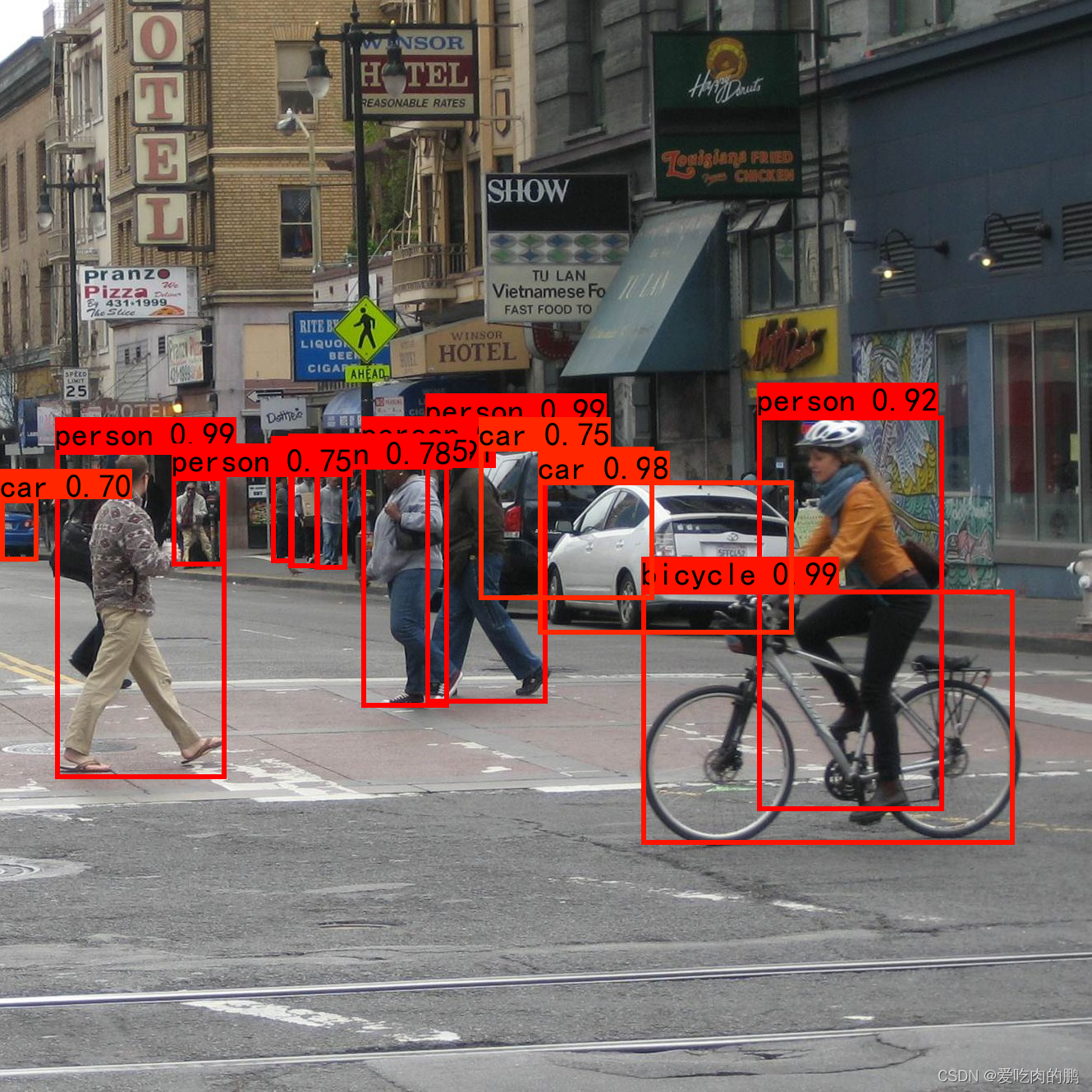
剪枝后的预测结果
在coco数据集上,剪枝前后的参数量输出如下:
Params: 64363101 => 60438323
正确的剪枝后会打印出以下信息【如果有类似的信息就是可以正常剪枝,如果没出现,说明你剪的不对】:
[ <DEP: prune_conv => prune_conv on conv2.2.conv (Conv2d(615, 512, kernel_size=(1, 1), stride=(1, 1), bias=False))>, Index=[1, 2, 3, 4, 7, 9, 15, 16, 17, 18, 23, 24, 35, 39, 42, 45, 46, 53, 54, 58, 62, 63, 65, 70, 73, 75, 81, 84, 88, 90, 97, 101, 102, 106, 109, 111, 112, 113, 116, 119, 124, 127, 132, 133, 135, 138, 140, 141, 143, 145, 148, 149, 150, 157, 159, 161, 163, 166, 168, 169, 170, 172, 174, 176, 177, 179, 180, 181, 182, 185, 186, 187, 189, 191, 193, 196, 200, 202, 207, 210, 211, 216, 217, 220, 222, 223, 225, 226, 228, 233, 234, 236, 238, 242, 243, 245, 246, 247, 248, 249, 251, 253, 254, 255, 256, 257, 266, 267, 270, 271, 279, 280, 284, 287, 288, 291, 295, 299, 301, 302, 305, 306, 307, 309, 311, 314, 316, 319, 325, 326, 328, 331, 333, 341, 342, 344, 345, 346, 348, 349, 352, 355, 356, 357, 361, 371, 372, 374, 375, 379, 381, 385, 388, 391, 394, 395, 399, 401, 403, 406, 408, 410, 414, 415, 418, 421, 425, 430, 432, 433, 434, 438, 439, 440, 444, 445, 448, 449, 452, 453, 461, 465, 467, 468, 469, 473, 475, 479, 480, 481, 482, 485, 487, 492, 493, 495, 497, 499, 504, 505, 507, 508, 510, 511], NumPruned=125460]
[ <DEP: prune_conv => prune_batchnorm on conv2.2.bn (BatchNorm2d(512, eps=1e-05, momentum=0.1, affine=True, track_running_stats=True))>, Index=[1, 2, 3, 4, 7, 9, 15, 16, 17, 18, 23, 24, 35, 39, 42, 45, 46, 53, 54, 58, 62, 63, 65, 70, 73, 75, 81, 84, 88, 90, 97, 101, 102, 106, 109, 111, 112, 113, 116, 119, 124, 127, 132, 133, 135, 138, 140, 141, 143, 145, 148, 149, 150, 157, 159, 161, 163, 166, 168, 169, 170, 172, 174, 176, 177, 179, 180, 181, 182, 185, 186, 187, 189, 191, 193, 196, 200, 202, 207, 210, 211, 216, 217, 220, 222, 223, 225, 226, 228, 233, 234, 236, 238, 242, 243, 245, 246, 247, 248, 249, 251, 253, 254, 255, 256, 257, 266, 267, 270, 271, 279, 280, 284, 287, 288, 291, 295, 299, 301, 302, 305, 306, 307, 309, 311, 314, 316, 319, 325, 326, 328, 331, 333, 341, 342, 344, 345, 346, 348, 349, 352, 355, 356, 357, 361, 371, 372, 374, 375, 379, 381, 385, 388, 391, 394, 395, 399, 401, 403, 406, 408, 410, 414, 415, 418, 421, 425, 430, 432, 433, 434, 438, 439, 440, 444, 445, 448, 449, 452, 453, 461, 465, 467, 468, 469, 473, 475, 479, 480, 481, 482, 485, 487, 492, 493, 495, 497, 499, 504, 505, 507, 508, 510, 511], NumPruned=408]
[ <DEP: prune_batchnorm => _prune_elementwise_op on _ElementWiseOp()>, Index=[1, 2, 3, 4, 7, 9, 15, 16, 17, 18, 23, 24, 35, 39, 42, 45, 46, 53, 54, 58, 62, 63, 65, 70, 73, 75, 81, 84, 88, 90, 97, 101, 102, 106, 109, 111, 112, 113, 116, 119, 124, 127, 132, 133, 135, 138, 140, 141, 143, 145, 148, 149, 150, 157, 159, 161, 163, 166, 168, 169, 170, 172, 174, 176, 177, 179, 180, 181, 182, 185, 186, 187, 189, 191, 193, 196, 200, 202, 207, 210, 211, 216, 217, 220, 222, 223, 225, 226, 228, 233, 234, 236, 238, 242, 243, 245, 246, 247, 248, 249, 251, 253, 254, 255, 256, 257, 266, 267, 270, 271, 279, 280, 284, 287, 288, 291, 295, 299, 301, 302, 305, 306, 307, 309, 311, 314, 316, 319, 325, 326, 328, 331, 333, 341, 342, 344, 345, 346, 348, 349, 352, 355, 356, 357, 361, 371, 372, 374, 375, 379, 381, 385, 388, 391, 394, 395, 399, 401, 403, 406, 408, 410, 414, 415, 418, 421, 425, 430, 432, 433, 434, 438, 439, 440, 444, 445, 448, 449, 452, 453, 461, 465, 467, 468, 469, 473, 475, 479, 480, 481, 482, 485, 487, 492, 493, 495, 497, 499, 504, 505, 507, 508, 510, 511], NumPruned=0]
[ <DEP: _prune_elementwise_op => prune_related_conv on upsample1.upsample.0.conv (Conv2d(512, 256, kernel_size=(1, 1), stride=(1, 1), bias=False))>, Index=[1, 2, 3, 4, 7, 9, 15, 16, 17, 18, 23, 24, 35, 39, 42, 45, 46, 53, 54, 58, 62, 63, 65, 70, 73, 75, 81, 84, 88, 90, 97, 101, 102, 106, 109, 111, 112, 113, 116, 119, 124, 127, 132, 133, 135, 138, 140, 141, 143, 145, 148, 149, 150, 157, 159, 161, 163, 166, 168, 169, 170, 172, 174, 176, 177, 179, 180, 181, 182, 185, 186, 187, 189, 191, 193, 196, 200, 202, 207, 210, 211, 216, 217, 220, 222, 223, 225, 226, 228, 233, 234, 236, 238, 242, 243, 245, 246, 247, 248, 249, 251, 253, 254, 255, 256, 257, 266, 267, 270, 271, 279, 280, 284, 287, 288, 291, 295, 299, 301, 302, 305, 306, 307, 309, 311, 314, 316, 319, 325, 326, 328, 331, 333, 341, 342, 344, 345, 346, 348, 349, 352, 355, 356, 357, 361, 371, 372, 374, 375, 379, 381, 385, 388, 391, 394, 395, 399, 401, 403, 406, 408, 410, 414, 415, 418, 421, 425, 430, 432, 433, 434, 438, 439, 440, 444, 445, 448, 449, 452, 453, 461, 465, 467, 468, 469, 473, 475, 479, 480, 481, 482, 485, 487, 492, 493, 495, 497, 499, 504, 505, 507, 508, 510, 511], NumPruned=52224]
[ <DEP: _prune_elementwise_op => _prune_concat on _ConcatOp([0, 512, 1024])>, Index=[513, 514, 515, 516, 519, 521, 527, 528, 529, 530, 535, 536, 547, 551, 554, 557, 558, 565, 566, 570, 574, 575, 577, 582, 585, 587, 593, 596, 600, 602, 609, 613, 614, 618, 621, 623, 624, 625, 628, 631, 636, 639, 644, 645, 647, 650, 652, 653, 655, 657, 660, 661, 662, 669, 671, 673, 675, 678, 680, 681, 682, 684, 686, 688, 689, 691, 692, 693, 694, 697, 698, 699, 701, 703, 705, 708, 712, 714, 719, 722, 723, 728, 729, 732, 734, 735, 737, 738, 740, 745, 746, 748, 750, 754, 755, 757, 758, 759, 760, 761, 763, 765, 766, 767, 768, 769, 778, 779, 782, 783, 791, 792, 796, 799, 800, 803, 807, 811, 813, 814, 817, 818, 819, 821, 823, 826, 828, 831, 837, 838, 840, 843, 845, 853, 854, 856, 857, 858, 860, 861, 864, 867, 868, 869, 873, 883, 884, 886, 887, 891, 893, 897, 900, 903, 906, 907, 911, 913, 915, 918, 920, 922, 926, 927, 930, 933, 937, 942, 944, 945, 946, 950, 951, 952, 956, 957, 960, 961, 964, 965, 973, 977, 979, 980, 981, 985, 987, 991, 992, 993, 994, 997, 999, 1004, 1005, 1007, 1009, 1011, 1016, 1017, 1019, 1020, 1022, 1023], NumPruned=0]
[ <DEP: _prune_concat => prune_related_conv on make_five_conv4.0.conv (Conv2d(1024, 512, kernel_size=(1, 1), stride=(1, 1), bias=False))>, Index=[513, 514, 515, 516, 519, 521, 527, 528, 529, 530, 535, 536, 547, 551, 554, 557, 558, 565, 566, 570, 574, 575, 577, 582, 585, 587, 593, 596, 600, 602, 609, 613, 614, 618, 621, 623, 624, 625, 628, 631, 636, 639, 644, 645, 647, 650, 652, 653, 655, 657, 660, 661, 662, 669, 671, 673, 675, 678, 680, 681, 682, 684, 686, 688, 689, 691, 692, 693, 694, 697, 698, 699, 701, 703, 705, 708, 712, 714, 719, 722, 723, 728, 729, 732, 734, 735, 737, 738, 740, 745, 746, 748, 750, 754, 755, 757, 758, 759, 760, 761, 763, 765, 766, 767, 768, 769, 778, 779, 782, 783, 791, 792, 796, 799, 800, 803, 807, 811, 813, 814, 817, 818, 819, 821, 823, 826, 828, 831, 837, 838, 840, 843, 845, 853, 854, 856, 857, 858, 860, 861, 864, 867, 868, 869, 873, 883, 884, 886, 887, 891, 893, 897, 900, 903, 906, 907, 911, 913, 915, 918, 920, 922, 926, 927, 930, 933, 937, 942, 944, 945, 946, 950, 951, 952, 956, 957, 960, 961, 964, 965, 973, 977, 979, 980, 981, 985, 987, 991, 992, 993, 994, 997, 999, 1004, 1005, 1007, 1009, 1011, 1016, 1017, 1019, 1020, 1022, 1023], NumPruned=104448]
282540 parameters will be pruned
代码
2022.06.09已对项目更新:更新说明,对项目所有功能进行了整合,加入了剪枝后的训练部分,具体使用详见代码中的readme.md
代码地址:https://github.com/YINYIPENG-EN/Pruning_for_yolov4.git
权重链接: 链接:百度云盘 提取码:yypn
本文内容由网友自发贡献,版权归原作者所有,本站不承担相应法律责任。如您发现有涉嫌抄袭侵权的内容,请联系:hwhale#tublm.com(使用前将#替换为@)